Overview

In this project, I built a cloth model using masses and springs. Then, I simulated cloth movement and calculated forces using numerical integration. I also handled collisions with other objects (e.g. sphere) and self-collisions. Lastly, I added shaders. Combined, these parts form a real-time cloth simulator.

Part 1: Masses and springs

In part 1, I implemented a cloth model using point masses and springs. To implement this model, I first constructed an evenly spaced grid of point masses based on the num_width_points and num_height_points. Then, I set the (x,y,z) coordinates of each point pass, where specific coordinate values depended on the orientation of the cloth. For example, horizontal cloth had a y coordinate of 1 (the cloth is essentially flat) while vertical cloth had a small offset applied to its z coordinate (this creates the illusion that a vertical cloth is not completely straight). Finally, I added springs and applied structural, shear, and bending constraints to make the cloth look more realistic.

The specs do a good job explaining when the spring constraints exist/don't exist. From the specs:

• Structural constraints exist between a point mass and the point mass to its left as well as the point mass above it.
• Shearing constraints exist between a point mass and the point mass to its diagonal upper left as well as the point mass to its diagonal upper right.
• Bending constraints exist between a point mass and the point mass two away to its left as well as the point mass two above it.

Below are some screenshots of pinned2.json from two viewing angles where you can see the cloth wireframe to show the structure of your point masses. I also show the wireframe without any shearing constraints, with only shearing constraints, and with all constraints.

Part 2: Simulation via numerical integration

In part 2, I implemented cloth movement by calculating and applying forces at each point mass. I computed external forces by using Newton’s 2nd Law, F = ma (plugging in the variables external_accelerations for a and mass for m). Then, I computed spring correction forces by applying Hooke’s law on springs that do not have a disabled constraint type. After calculating all the forces at each point mass, I had to implement an integration method to compute the new position of each point mass due to force. For this project, I utilized Verlet integration as suggested in the specs. Verlet integration is an explicit integrator that is derived from positional changes based on velocity and acceleration. To approximate v*dt, the integrator uses x(t) – x(t-dt), where x(t-dt) equals the position from the previous time step. In addition to this substitution of v*dt, I added a damping factor to simulate the friction that occurs during cloth movement. After calculating positional changes, I had to implement an update technique that ensures the springs will not get deformed too much. Essentially, at every time step, I check to make sure the springs defined by two unpinned point masses are stretching more than 10% of its resting length (rest_length variable).

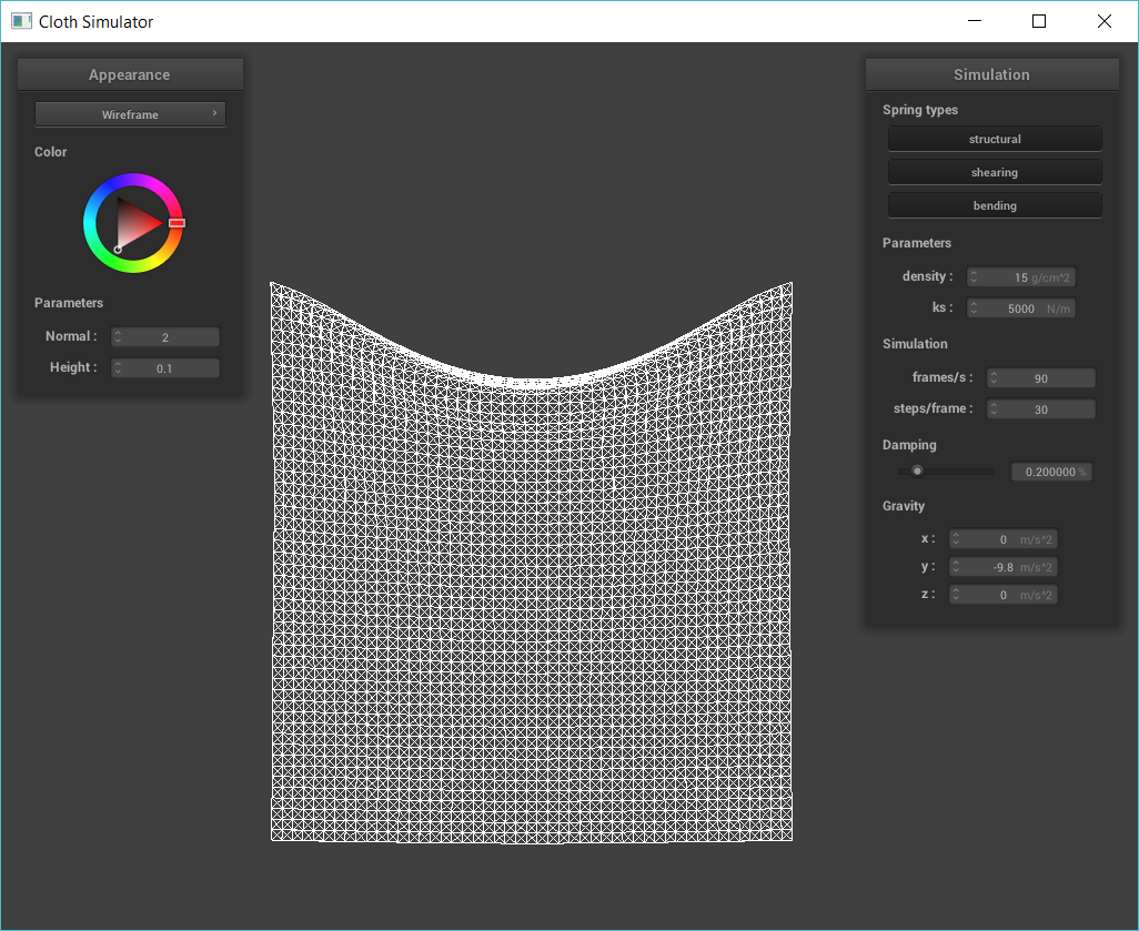
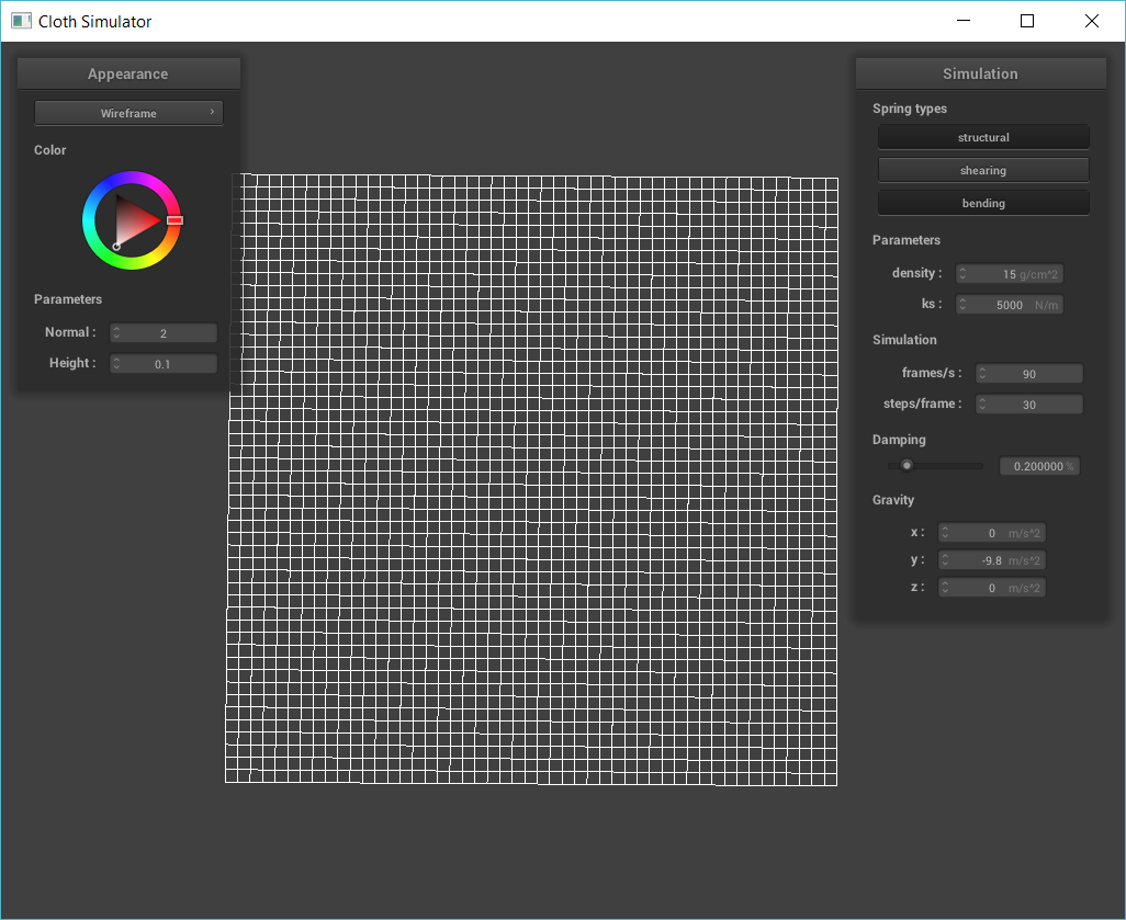
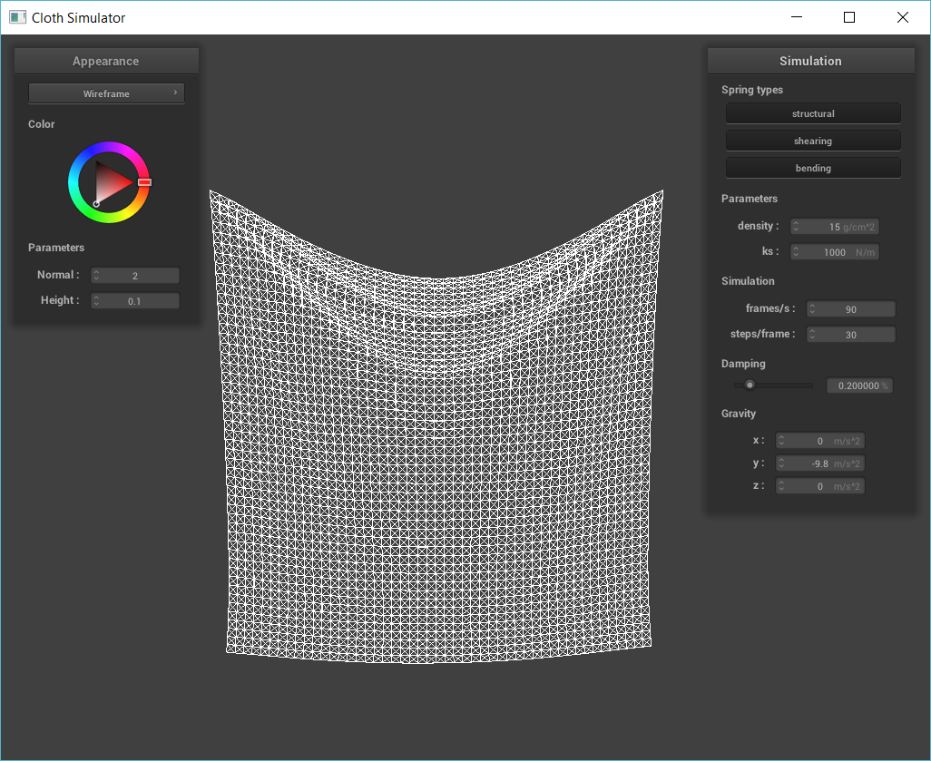
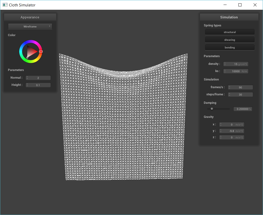
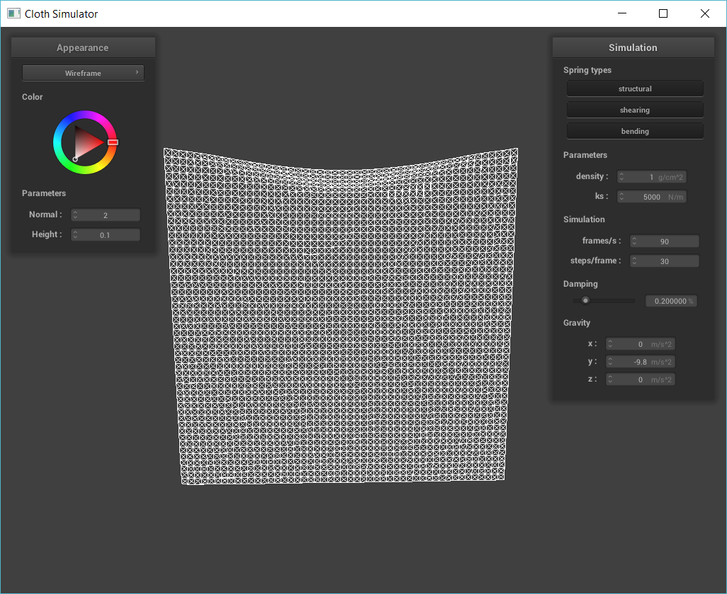
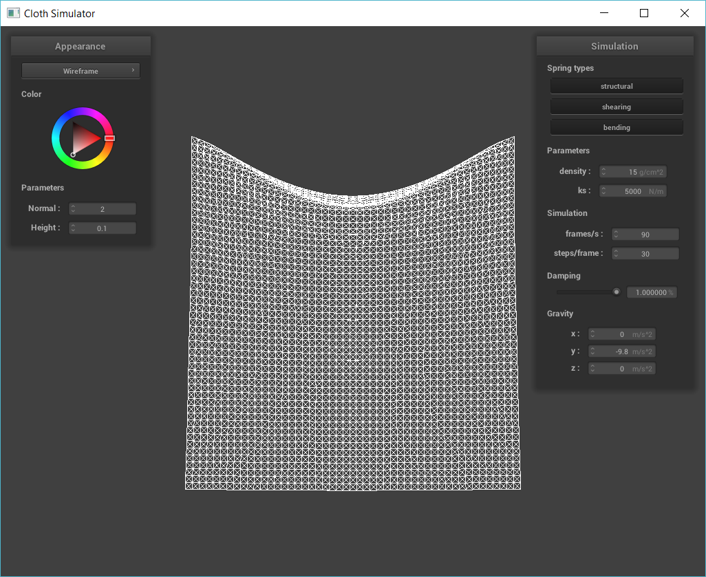
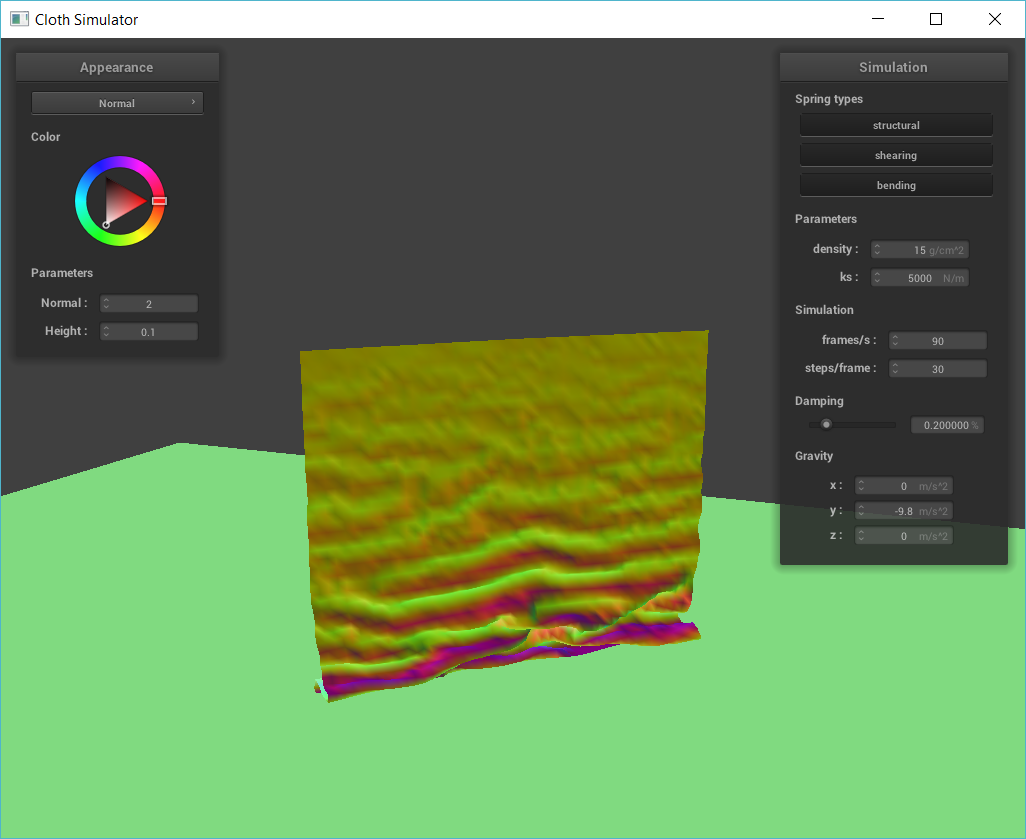
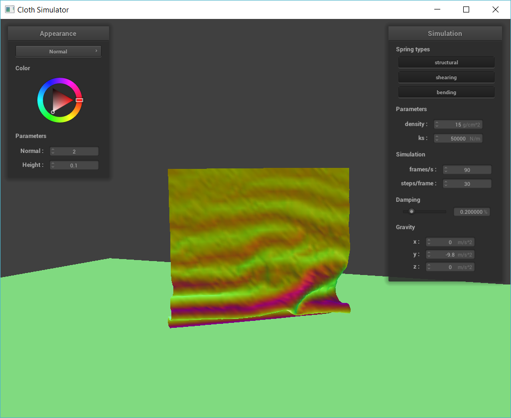
Below I experiment with the parameters in the simulation. First, I'll show images with varying spring constant ks.

As you can see above, the cloth with lower ks (1000 N/m) is more droopy and elastic while the higher ks cloths (5000 and 10000 N/m) are stiffer. This stiffness of the high ks cloths is particularly noticeable when the cloth is falling down and exhibit very little elastic behavior. On the other hand, from start to rest, the cloth with lower ks is significantly more elastic; specifically, the low ks cloth appears wrinkly and moves shakily while the cloth with higher ks are more resistant to movement, noticeably tighter, and less droppy. This is why the cloth with the highest ks (10000 N/m) is the least droopy (evident at the center) in its final resting position. Intuitively, what is happening is that when the ks increases, the springs don't need to stretch as much to counteract the gravitational force. When ks decreases, the springs need to stretch more to counteract the gravitational force. Thus, compared to the default density cloth, the cloth with ks = 10000 is stiffer and less droopy (especially evident at the top center of the cloth). Compared to the default density cloth, the cloth with ks = 1000 is more elastic and droopy.

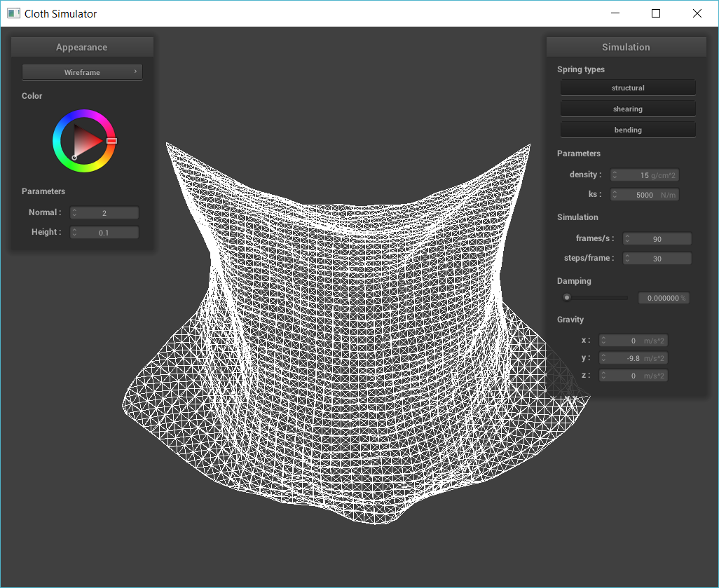
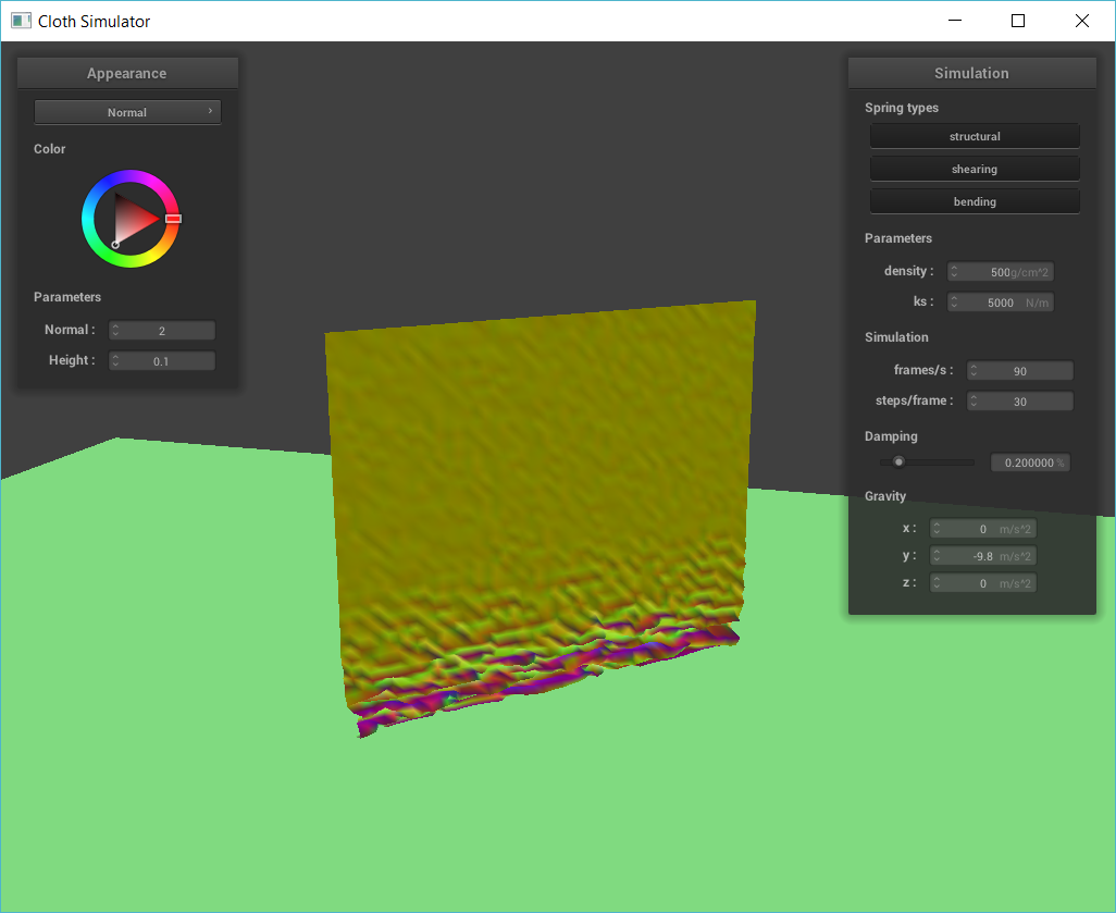
Below are images depicting the effects of changing the density.

Above, the higher the density, the more droopy/elastic the cloth is. The lower the density, the less droopy/elastic it is. The behavior is the exact opposite of increasing/decreasing ks. Intuitively, this is because increasing density makes the point mass heavier. Thus, the spring force has less of an effect on these heavier masses and the cloth is dominated by gravitational force and droops lower. When the density is decreased, the point masses are lighter and the spring forces have a stronger effect on cloth, meaning the cloth is less dominated by gravitational force and not as droopy. In summary, compared to the default density cloth, the cloth with a density of 1g/cm^2 is stiffer and less droopy (especially evident at the top of the cloth). Compared to the default density cloth, the cloth with a density of 40g/cm^2 is more elastic and droopy.

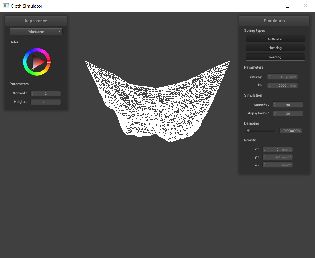
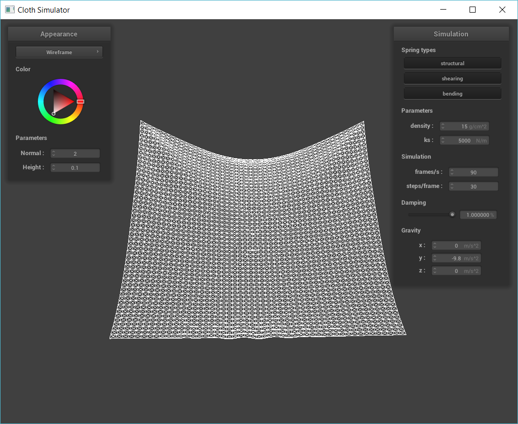
Below are images depicting the effects of changing damping.

Above, the higher the damping, the slower the cloth falls. Once the cloth with high damping reaches the equilibrium position, the cloth pretty much stabilizes and remains at that position. Intutively, what is happening is that increasing the damping factor adds friction, heat loss, etc, to the system, decreasing the net amount of energy in the cloth's movement and allowing the cloth with high damping to stop. Notice there is also less cloth movement/deformation for the high damping cloth during the actual falling phase. This is also due to higher net energy loss that results from higher damping. On the other hand, decreasing the damping causes the cloth to fall quicker and behave very elastically during the fall. In fact, due to the lack of friction, the cloth with 0% damping actually swings past the equilibrium point. Thus, the cloth with high damping (1%) is more resistant to movement and when it has low damping (0%), the cloth is less resistant to movement. The cloth with low damping takes longer to stop at its equilibrium position. The cloth with default damping (0.2%) falls slower (in terms of velocity, not time to reach equilibrium) than the cloth with low damping and faster than the cloth with high damping.

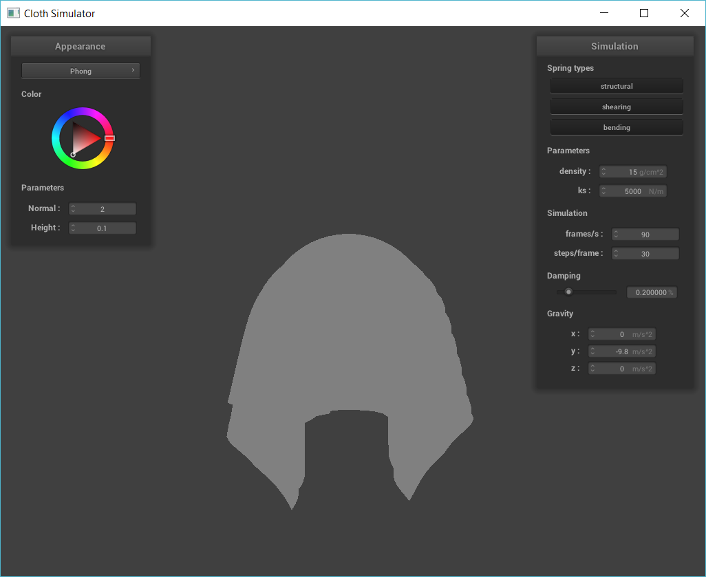
Below is a screenshot of my shaded cloth from scene/pinned4.json in its final resting state. I used the default parameters.

Part 3: Handling collisions with other objects

In part 3, I handled cloth collision with spheres and planes. For sphere collision, I checked if there was a collision and adjusted the last_position using a correction vector. To get the correction vector, I found the tangent. To calculate the tangent, I found the direction of the ray from the sphere's center to the particle with pm.position - origin, multiplied by radius, and added to origin to get the point on the sphere's surface. Finally, the correction vector equals tangent minus point mass's last position. The correction vector transforms the point mass’s last position to the point mass position tangent to the sphere. For plane collision, I replicated the same process as sphere collision. First, I check if there is actually a collision. Then, I multiply dist*normal.unit() and add to last_position to get tangent. I calculated the correction vector and set the point mass’s position to last_position adjusted by the correction vector. In this case, the correction vector transforms the point mass’ last position to a point slightly above (using a small offset value) the point mass position tangent to the plane. Also, for both sphere and plane collision, I scale down the final positions to account for friction.

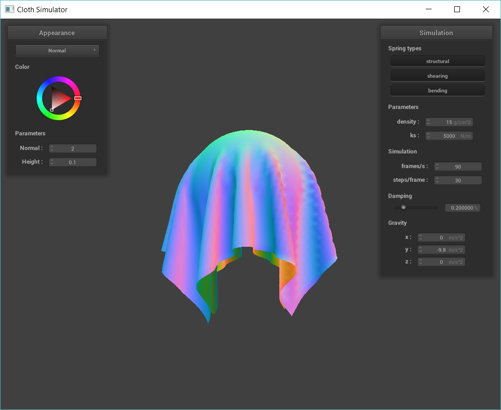
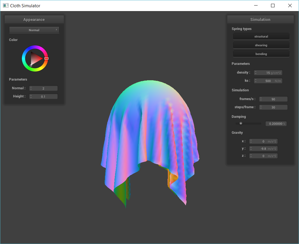
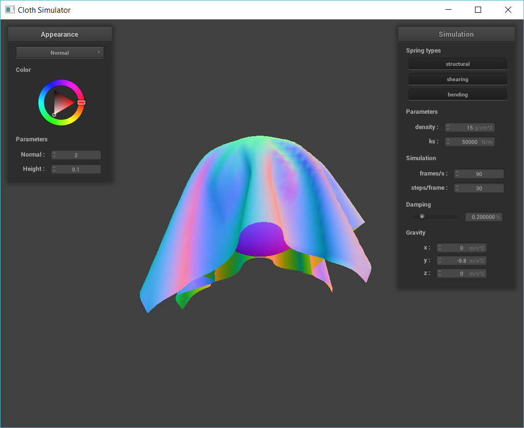
Below are screenshots of my shaded cloth from scene/sphere.json in its final resting state on the sphere using default ks = 5000, ks = 500, and ks = 50000. Below the images, I will describe their differences.

As you can see above, the cloth with the highest ks value (50000) is the most spread out on the sphere. The cloth with the lowest ks value (500) is the least spread out (most droopy) and the cloth with the default ks (5000) has a spread that is in between the cloths with ks = 500 and 50000. These results occur because increasing ks increases the stiffness of the cloth, and, the stiffer the cloth, the less drapey/spread out the cloth is when it is on the sphere. Another way to phrase is would be: higher ks means the cloth is able to retain more of its original shape. Lower ks means the cloth is able to deform/droop more.

Below is a screenshot of my shaded cloth lying peacefully at rest on the plane. I decided to use Texture Mapping to make the scene more interesting.

Part 4: Handling self-collisions

In part 4, I implemented cloth self-collision. Before, the cloth would behave unrealistically when collapsing upon itself. To make the cloth self-collision seem more realistic, I computed an additional force that is applied to two point masses when the two masses are within a certain threshold distance away from each other. Since there are n point masses to check on the grid, it would be a O(n^2) solution if I naively loop through all pairs of point masses. Thus, to make this check more optimal, I utilized spatial hashing. Spatial hashing essentially partitions the space into boxes (kind of similar to the idea of bounding volume hierarchy from previous projects). Then, I only need to check if a point within a box is within that threshold distance with another point within the box. If two points are within that threshold distance, I apply a repulsive collision force (implemented through a correction vector) so that the pair of masses are >= 2* thickness distance (less than 2*thickness distance is the threshold) apart.

Below are 3 screenshots that document how the cloth falls and folds on itself, starting with an early, initial self-collision and ending with the cloth at a more restful state.

Below I vary the density of the cloth, which affects the behavior of the cloth as it falls on itself.

As you can see above, the cloth with the highest density (500g/cm^2) has significantly more folds near the bottom when falling down. The cloth with the lowest density has significantly less folds near the bottom and the cloth with the default density has a number of folds that is in between. Intuitively, cloths with higher densities expriences a larger gravitational force (Fg = mg where g is gravity). This is why the cloth with the highest density seems to pulled downwards, with noticeably less horizontal movement near the top of the cloth as it is falling. The cloth with lower density is more elastic and both top and bottom of the cloth experiences wavy folds.

Below I vary the ks of the cloth, which affects the behavior of the cloth as it falls on itself.

As you can see above, the cloth with the the highest ks (50000 N/m) has the least number of folds. This is because increasing the ks, increases the stiffness of the cloth, which would make it have less folds. The cloth with the lowest ks (100 N/m) has significantly more folds. This is because the cloth is the most elastic. Essentially, the same things from the varying density part can be said here (except the effect of high ks corresponds to the effect of a low density).

Part 5: Shaders

In part 5, I implemented shaders, specifically diffuse shading, Blinn-Phong shading, texture mapping, displacement and bump mapping, and environment-mapped reflections.

Shaders are user-defined programs that run in parallel on the GPU and allows one to modify/execute certain steps in the rasterization pipeline (recall the rasterization pipeline consists of vertex processing, triangle processing, rasterization, fragment processing, and framebuffer operations). Vertex shaders modify the triangle processing stage, allowing one to change the position of individual vertices and their position/normal vectors. Fragment shaders modify the fragment processing stage and allow one to compute a color and create shaded fragments. To combine vertex and fragment shades, we take the output of the vertex shader and feed it into the fragment shader, and the fragment shader outputs a color. The order (vertex -> fragment) makes sense because the triangle processing stage occurs prior to the fragment processing stage.

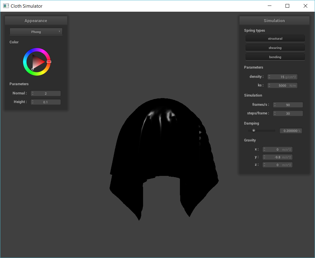
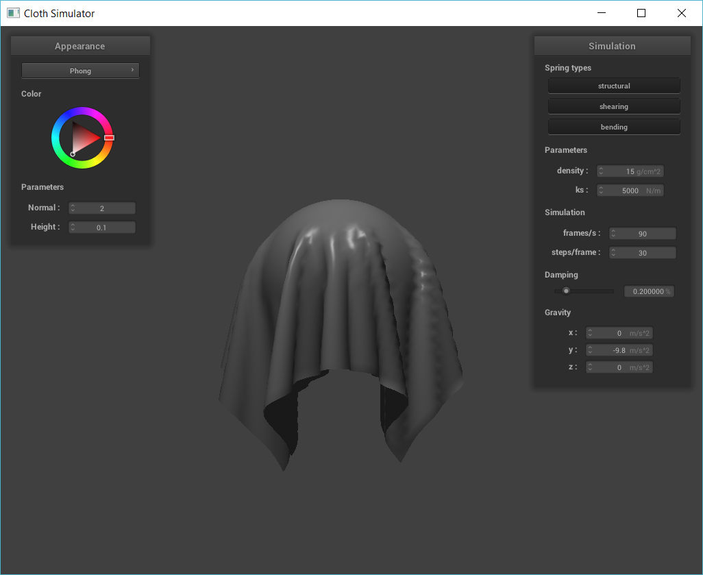
Blinn-Phong shading is a lighting model that sums up the ambient, specular, and diffuse lighting component to create physically plausible, fast shading of objects. There are many adjustable parameters that affect the final result of the Blinn-Phone model, such as the reflection coefficient for ambient, specular, and diffuse, the intensity of light (e.g. I_a), and shininess (e.g. the higher the p, the less shiny it is) of the object. Importantly, the Blinn-Phon model uses a halfway vector, which is a unit vector halfway between view and light direction, to get the specular contribution. The closer the halfway vector is to the surface normal vector, the larger the specular contribution.

Below are screenshots of my Blinn-Phong shader outputting only the ambient component, only the diffuse component, only the specular component, and one using the entire Blinn-Phong model.

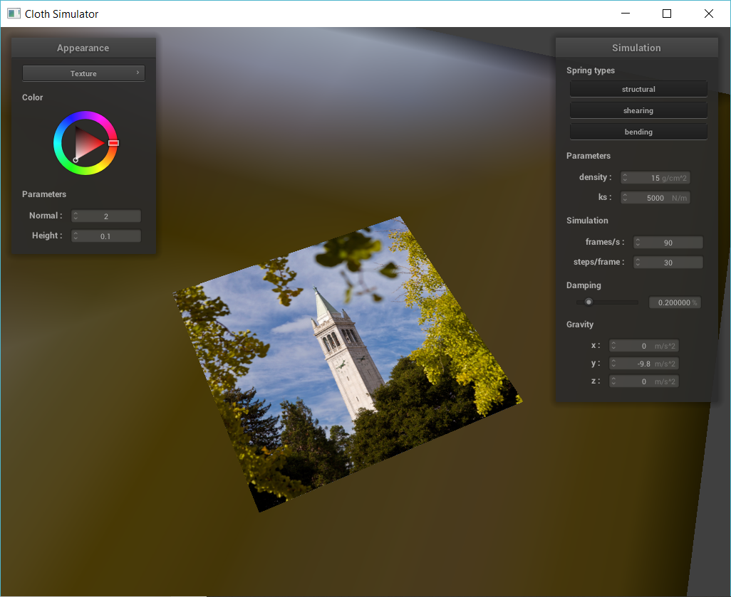
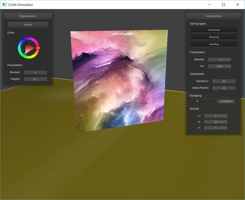
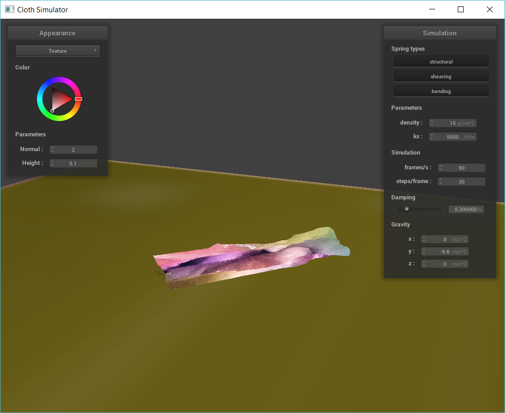
Below are two screenshots of my texture mapping shader using my own custom texture (image of a galaxy!).

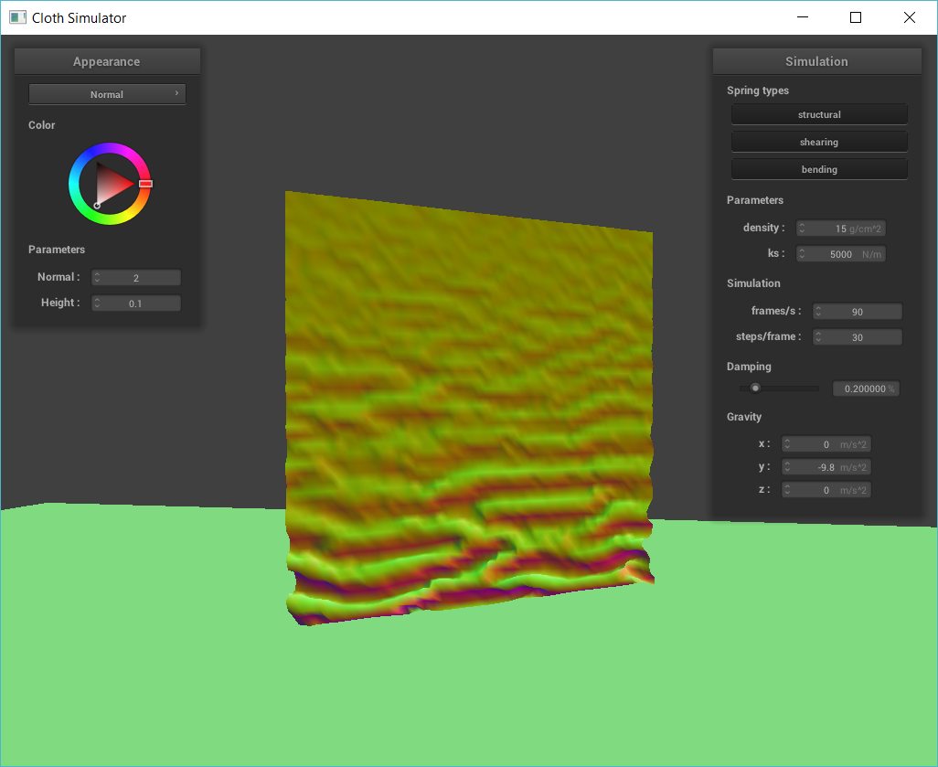
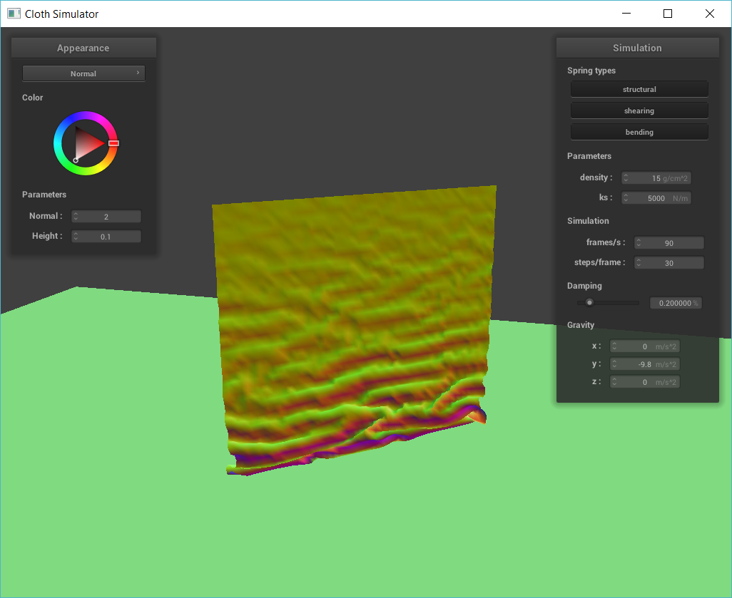
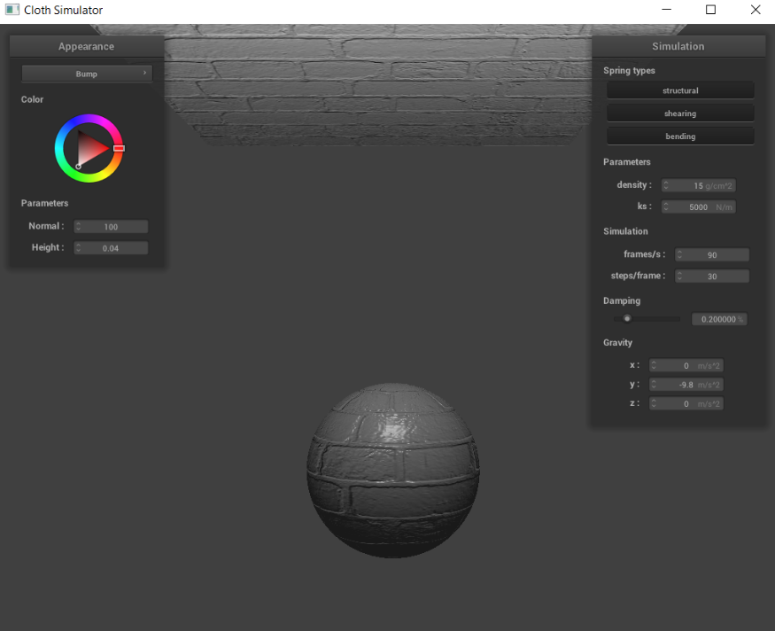
Below are screenshots of bump mapping on the cloth and sphere using texture_3 (stone brick). I used a Normal = 100 and Height = 0.04 for all the images below.

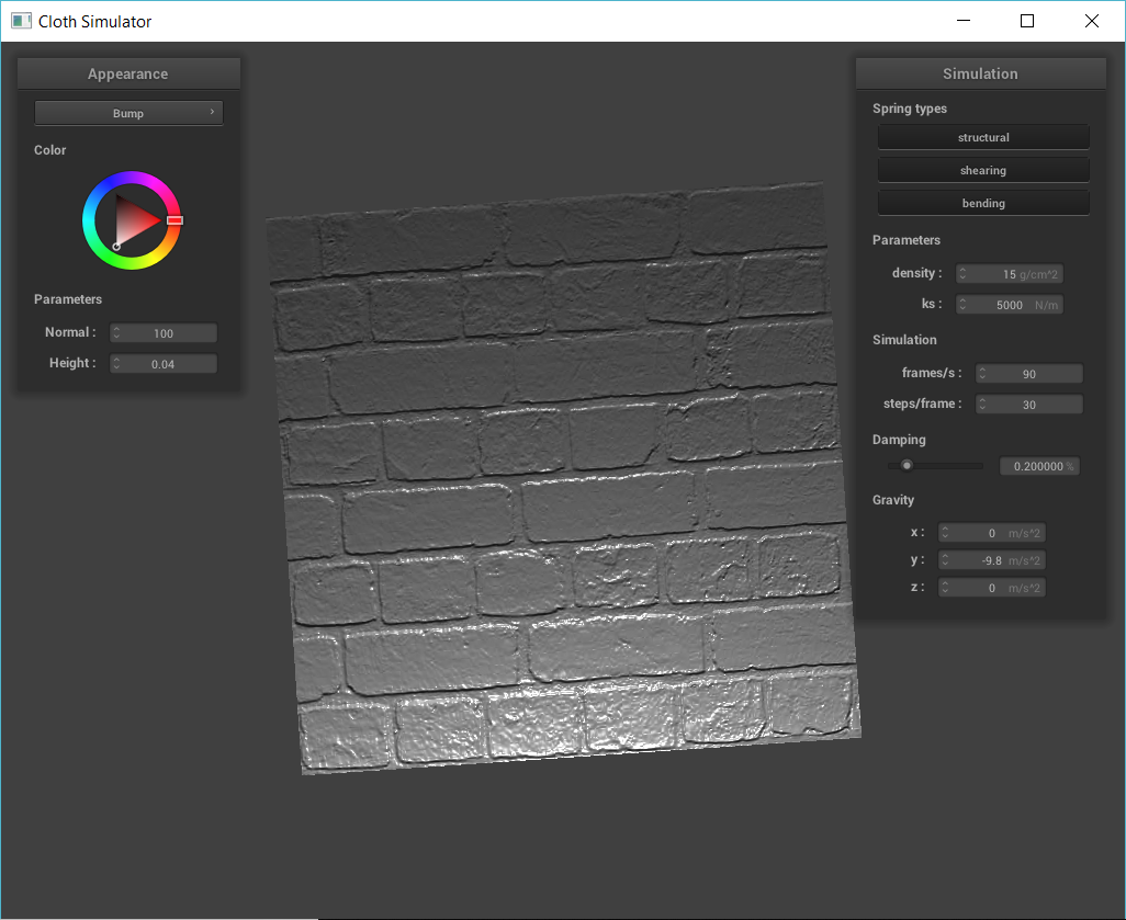
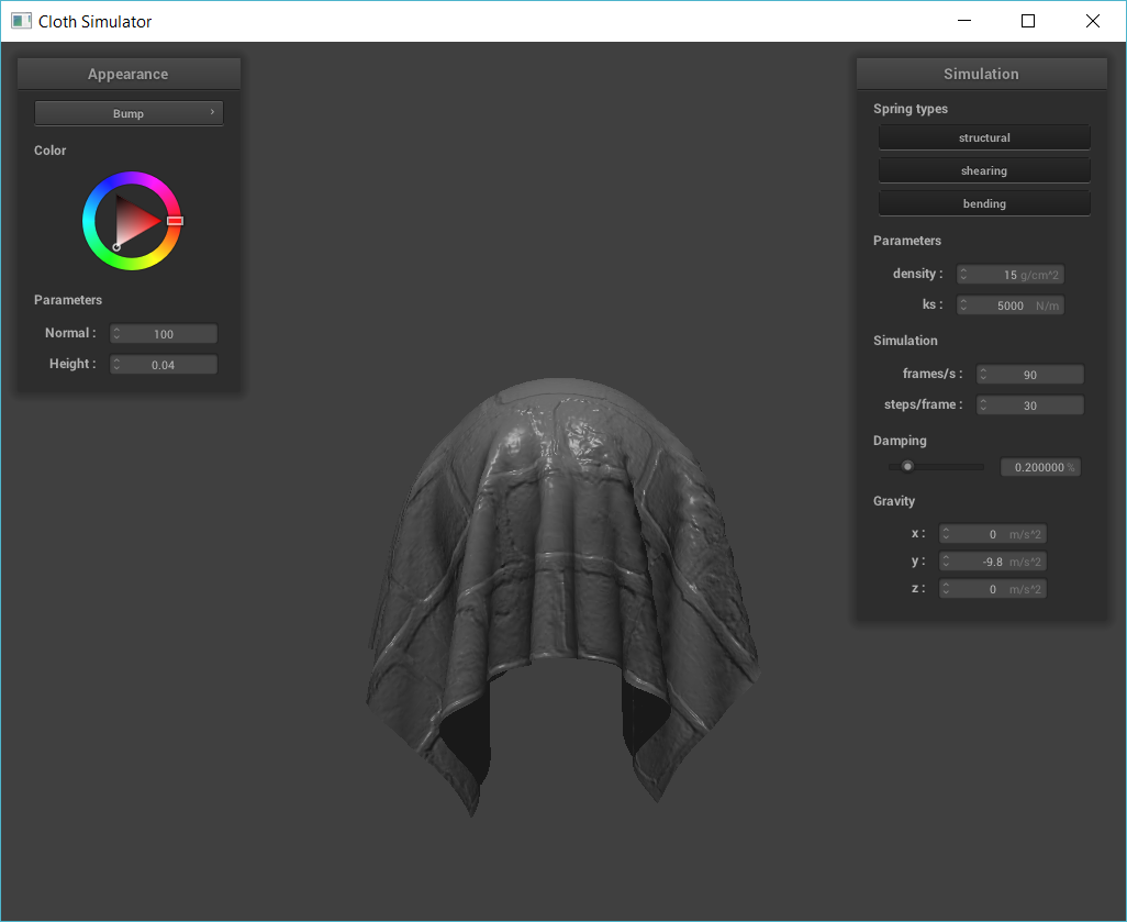
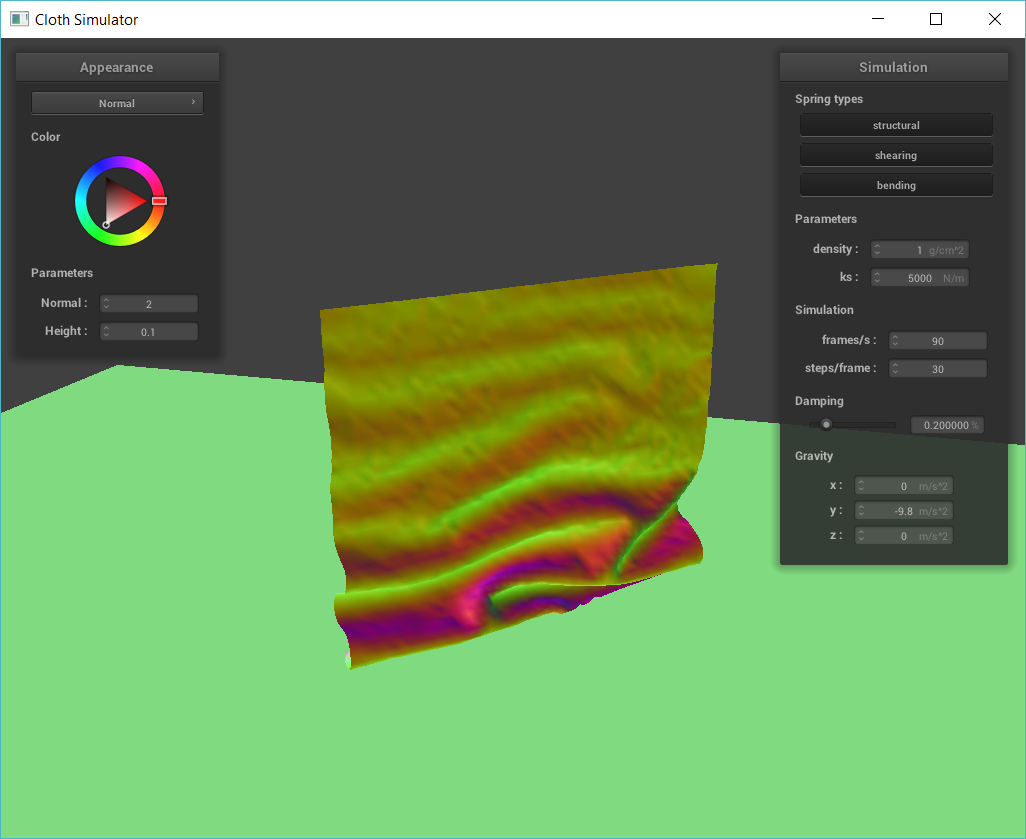
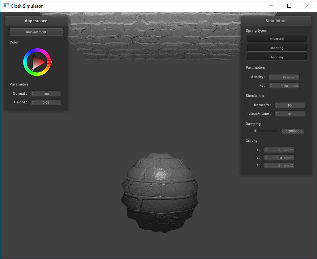
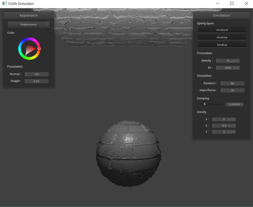
Below is a screenshot of displacement mapping on the sphere using texture_3 (stone brick).

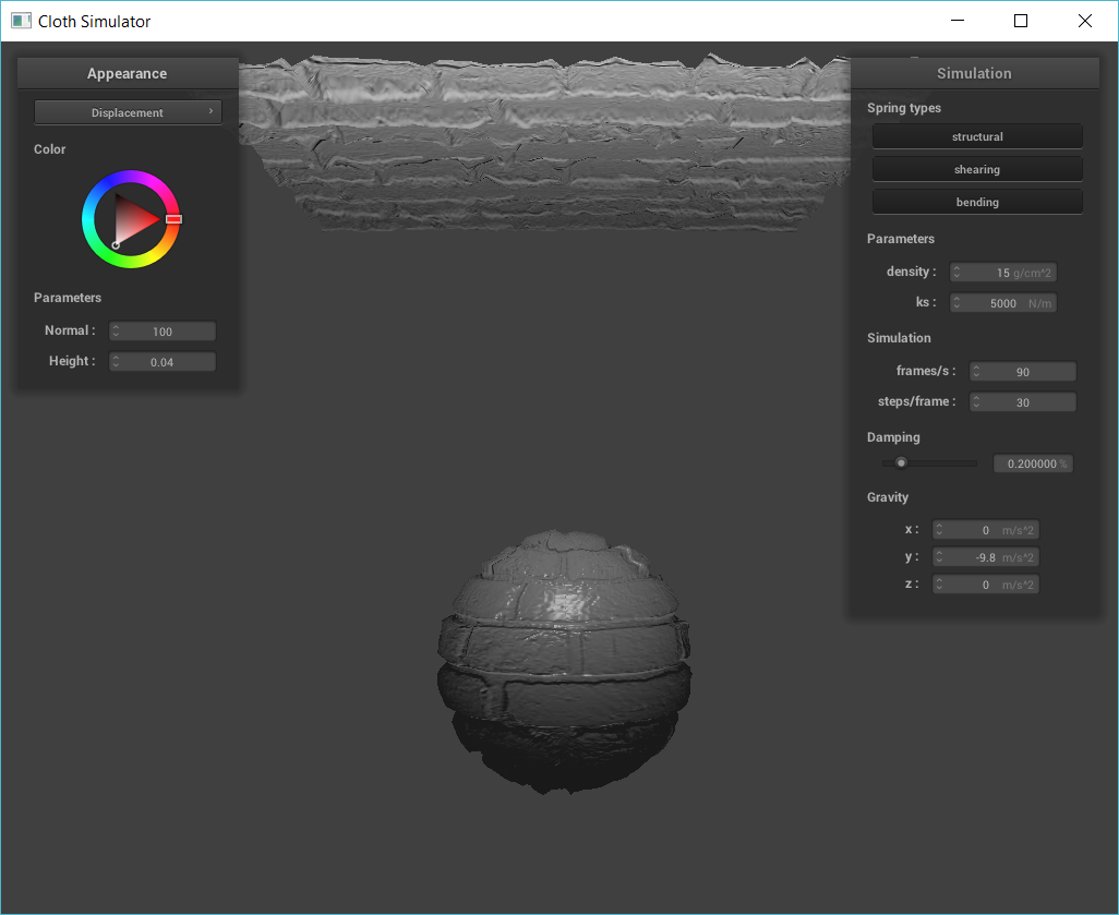
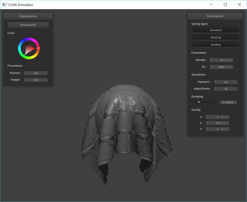
Now I will compare the two approaches and resulting renders. Bump and displacement mapping are extremely similar, except displacement mapping adds in an additional step of displacing the vertex positions. Bump mapping only modifes the normals of an object. Additionaly, in bump mapping, the texture is directly applied on the sphere, so there is no change in vertex positions of the object. On the other hand, displacement mapping modifies vertex positions to the height map and modifies normals to be consistent with the new vertex positions. Displacement mapping has more "bumpy" features because the surface is actually changing physically rather than just giving the illusion there are bumps.

Below I will show and compare how the two shaders react to the sphere by changing the sphere mesh's coarseness by using -o 16 -a 16 and then -o 128 -a 128.

As you can see above, changing coarseness does not have a very noticeable affect on bump mapping. This is because bump mapping is based on pixels rather than vertices. On the other hand, changing the coarseness affects displacement because diisplacement actually moves the vertices. The more/less details due to changes in coarseness is significantly more noticeable on the displacement sphere. With few vertices, the displacement sphere is not very detailed. However, with more vertices, there is more detail on the displacement sphere.

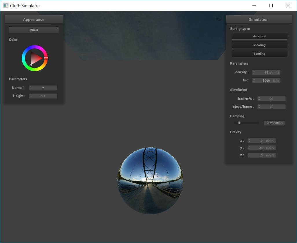
Below is a screenshot of my mirror shader on the cloth and on the sphere.

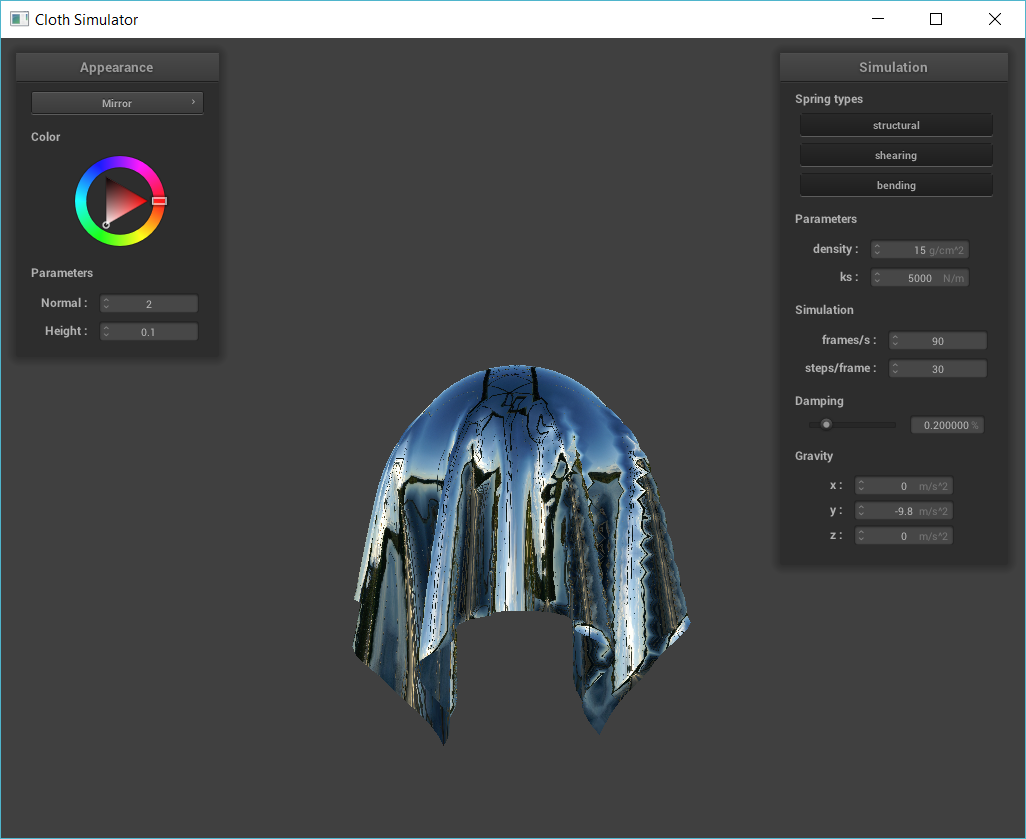
Extra credit: Below is my custom shader for extra credit. I implemented a dotted texture, where the dots are generated pseudo-randomly. I could not find a rand() function in GLSL, so I used a psuedo-random number generator. The generator used was fract(sin(dot(co.xy ,vec2(12.9898,78.233))) * 43758.5453), which returns a random number between 0 and 1 when given a 2d vector (source: http://www.science-and-fiction.org/rendering/noise.html). If the random number is < 0.5, I set all the k coefficients to 0.3. If the random number is >= 0.5, I set all the k coefficients to 0.9. This creates an interesting dynamic, dotted design; the dots appear to be moving at each time step due to the random behavior.