Overview

In this assignment, I built Bezier curves/surfaces using de Casteljau's algorithm and extensively used the half-edge data structure to manipulate meshes. In the last part, I implemented loop subdivison. The result of all these parts allow me to load and edit basic COLLADA mesh files. I learned how important it is to carefully keep track of all the pointers in the half-edge data structure. It is very easy to incorrectly assign a pointer when performing edge splits/flips.

Section I: Bezier Curves and Surfaces

Part 1: Bezier curves with 1D de Casteljau subdivision

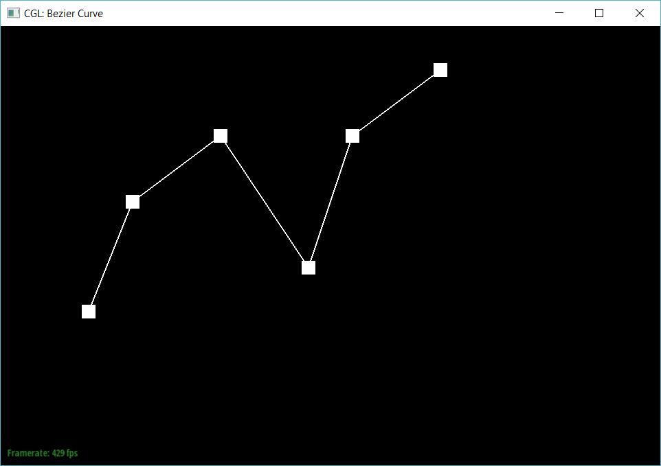
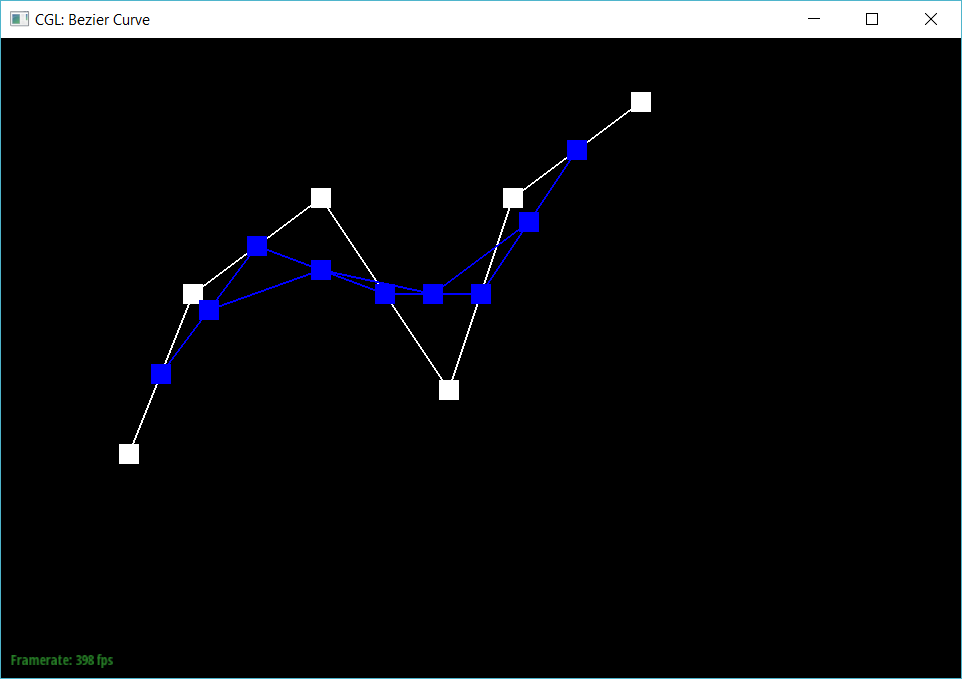
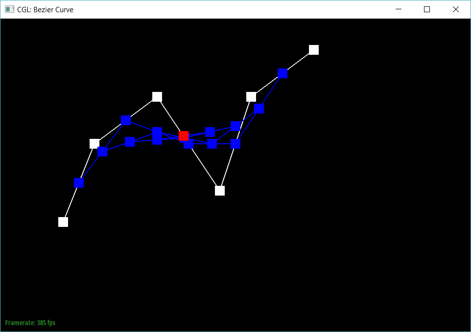
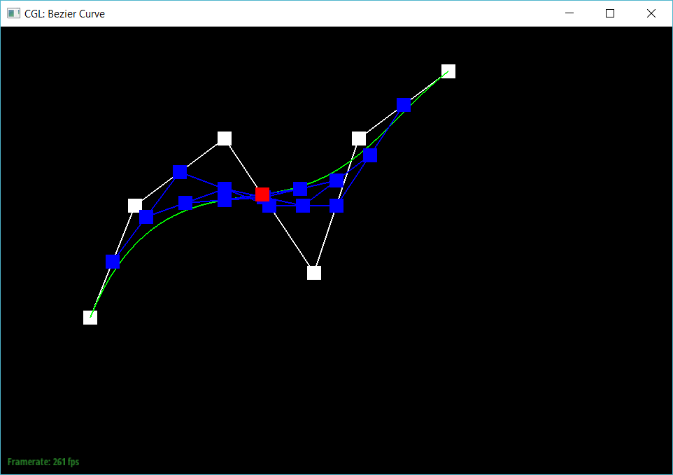
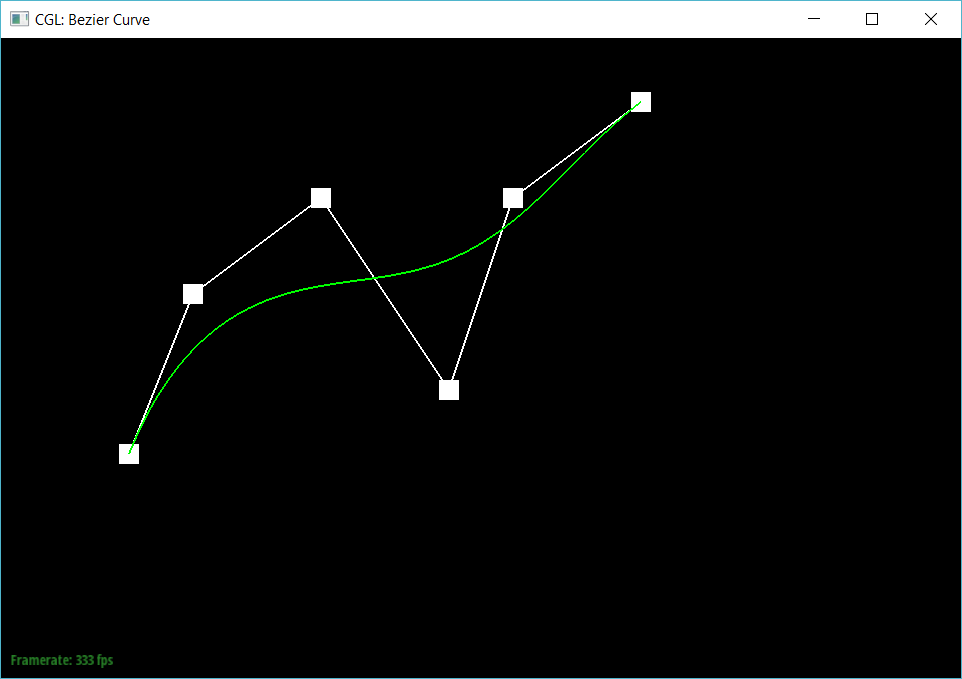
Given n control points, de Casteljau’s algorithm gives us a way to recursively subdivide the n-1 line segments between the control points and define interpolated points. For example, between points x0 and x1, we would define a point x0_1 at some position t along the line from x0. The variable t determines how far we are between x0 and x1; when t is 0, we’re at x0. When t is 1, we’re at the x1 end of the line segment. Similarly, we define more points by interpolating the rest of the control point pairs (adjacent control points). Critically, for all control point pairs, we define the interpolated point using the same value of t . The idea of this algorithm is that we just keep recursively interpolating points until we run out of line segments we can create from this method. In other words, we would keep creating a line segment between the adjacent interpolated points, and put a new interpolated point on that line segment. Ultimately, the final point we arrive at is a point on the Bezier curve.

I implemented a function that performs one step of the algorithm each time it is called. I first obtained the size of the most the recent level. Then, I determined the size of the new level by setting it equal to the size of the recent level minus one. Finally, I used the algebraic formula lerp(p_i, p_i+1, t) = (1 - t)p_i + (1−t)p_i+1 to find the interpolated point between each pair of adjacent points from the most recent level. This function can be called multiple times to get down to that last single evaluated point. Below are some images of a Bezier curve with 6 control points.

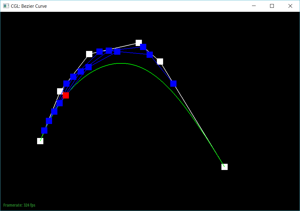
Below is a slightly different Bezier Curve

Part 2: Bezier surfaces with separable 1D de Casteljau subdivision

Before, in part 1, we had used n control points to define a Bezier curve. In part 2, we use an array of nxn control points to construct a Bezier curve. The idea is to take each of the n rows and interpret them each as a Bezier curve in one dimension (n). Then, we interpolate the corresponding values along each of the n Bezier curves to define a Bezier curve in the other dimension (v). The surface swept out by that second group of Bezier curves is the Bezier surface. I extended de Casteljau’s alogirthm to Bezier surfaces by applying the algorithm in two dimensions. To be more specific, I started by repeatedly calling the evaluated1d function (one row of control points at a time) in order to determine the initial set of Bezier curves in the u dimension. Then, to extend the Bezier curves to a Bezier surface, I evaluated the u points at parameter t in the v dimension. As a side note, the function know its reached the end position when the number of points evaluated in a recursive call is 1.

Section II: Sampling

Part 3: Average normals for half-edge meshes

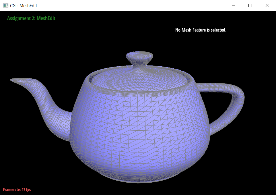
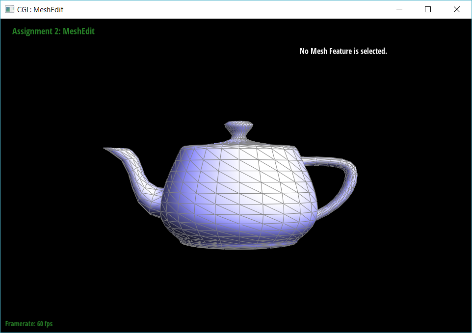
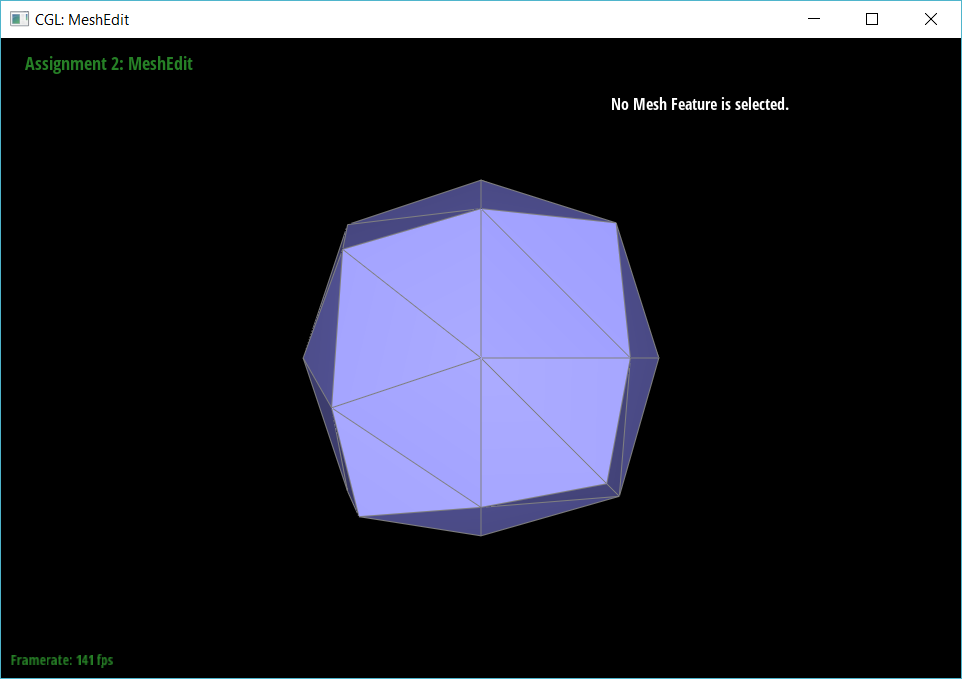
In part 3, I produced a more realistic (smoother) shading on the teapot by taking the area-weighted average normal vector at a vertex. I implemented this by starting out at the given vertex (e.g v0) and finding two other vertices (e.g. v1 and v2) on the same face/triangle. Then, I constructed two edges, edgeA and edgeB, by subtracting v1 with v0 and v2 with v1 respectively. Finally, I took the cross product of these two edges to get the area-weighted normal of the face. I continued this process for each face surrounding the vertex, adding the cross product to the “n” variable each time. Finally, after iterating through the faces, I return the re-normalized unit vector by calling n.unit().

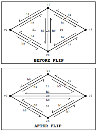
Part 4: Half-edge flip

In part 4, I implemented the half-edge flip operation by utilizing the Half-Edge data structure and reassigning various pointers to vertices, halfedges, faces, and edges in such a way that an edge gets flipped. This part looked straightforward on paper, but I knew it could get very confusing/buggy to implement. In order to efficiently complete this potentially “messy” task, I decided to draw out the diagrams before coding (the paper approach). Using CMU images as reference (provided by a TA on piazza), I first drew a diagram representing an edge before an edge flip. Then, I drew a diagram representing the edge after the flip. As you can see below, the elements (halfedge, vertex, edge, and face) are clearly labeled in the diagram, making it significantly easier to systematically reassign pointers. To actually implement this diagram in code, I simply created variables for every element in the diagram. Then, starting with the halfedges, I called setNeighbors on each halfedge (going from h0 to h9) and was able to set up the edge’s neighboring elements very efficiently. Using an ordered approach (going from h0 to h9) allowed me to keep track of what halfedges I had already changed. I used this same systematic, ordered approach when reassigning the vertices, edges, and faces. Using a systematic approach and drawing the diagrams on paper was crucial for me to complete this part efficiently and without any bugs

Part 5: Half-edge split

In part 5, I implemented the half-edge split operation. Similar to part 4, I utilized the Half-Edge data structure. However, now I had to add 3 new edges, 2 new triangles/faces, 1 new vertex, and 6 new halfedges to create the new elements that result from splitting an edge. I took the paper approach once again. I first drew out an edge before split (using the same “initial state” diagram from part 4). Then, I drew out the diagram after an edge split. This latter part was slightly more difficult because it involved introducing new elements to the diagram (new vertices, edges, etc.). I had to decide where to place the new elements. Thus, to make sure I was able to complete this part without any bugs, I came up with very clear labels/names for each new element in order to keep track of changes. For example, for the new halfedge I added to the right of h0, I named it h0right. For h0’s new twin, I called it h0twin. By clearly labeling these new elements, I was able to once again take a systematic, ordered approach (e.g. setting neighbors for each halfedge one at a time) and complete the task efficiently.

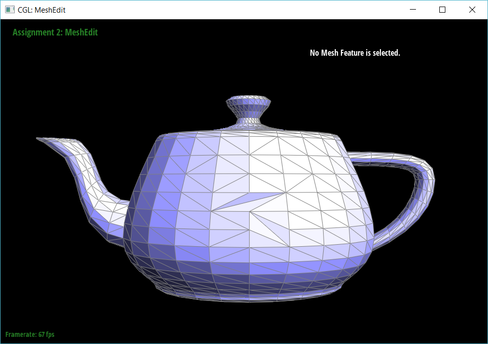
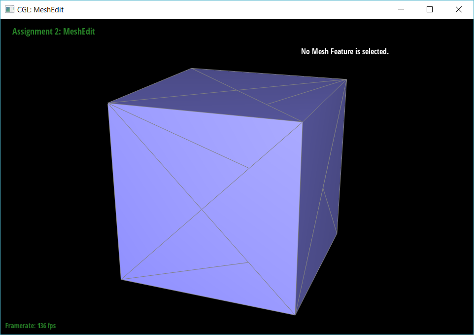
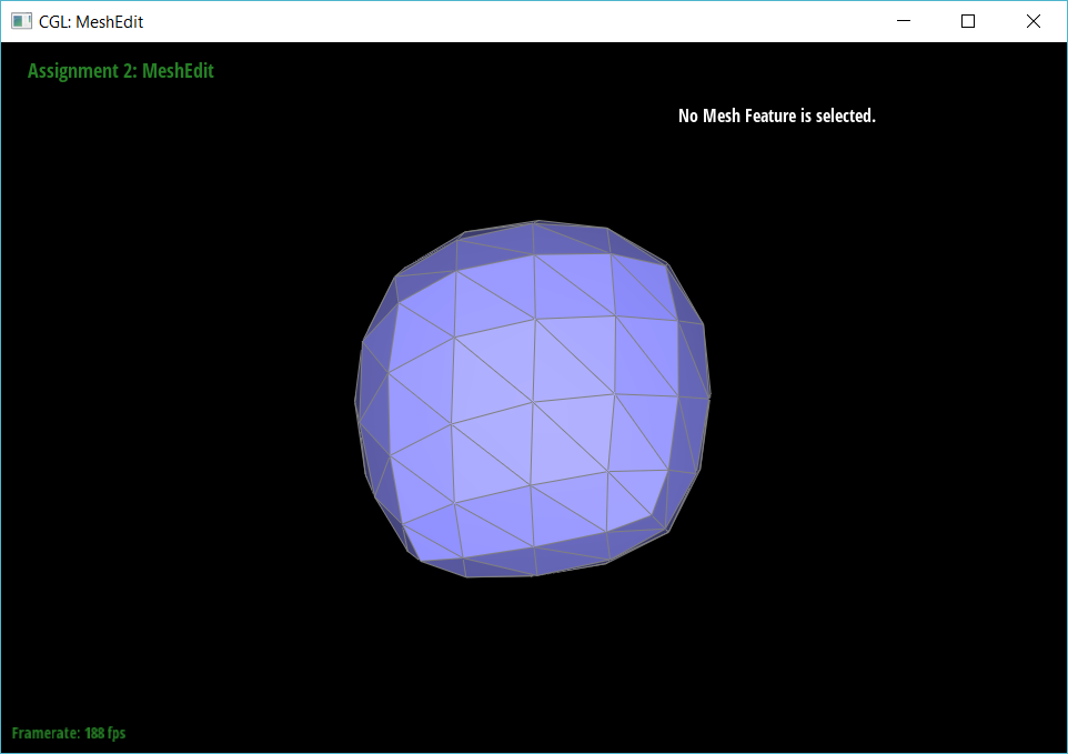
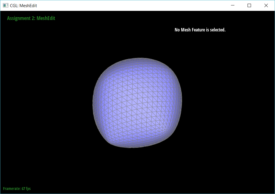
Part 6: Loop subdivision for mesh upsampling

In part 6, I implemented Loop subdivision. I started by calculating the new positions of all vertices in the original mesh. I did this by iterating through all the vertices and using the weighted positions of each vertices’ neighboring vertices (the exact weight used depends on the degree of the vertex). I stored all these new positions in Vertex::newPosition. The next step involved storing the new vertex positions associated with the edge midpoints. This involved using four neighboring vertices and applying weights according to the following formula: 3/8 * (A + B) + 1/8 * (C + D). I stored these newly created vertex positions in e->newPosition. Using the results from the prior step, I was able to split the edges from the original mesh. I made sure to only split the original edges by checking !e->halfedge()->vertex()->isNew && !e->halfedge()->twin()->vertex()->isNew. In other words, I only split edges with two end vertices that were not new. After splitting the edge and getting a new vertex, I assigned the new vertex position to newPosition, which was calculated in the prior step. Next, I flipped all edge that connected an old vertex with a new vertex. I carefully used two booleans to make sure that the new edge must be connecting exactly one old vertex and exactly one new vertex (only “old and new”/“new and old” return true) Finally, I iterated through all the vertices once again and set them equal to their newPosition. Below are some images of meshes after Loop subdivision.

To implement this without any bugs, I made sure I clearly understood the process before starting, and I worked on each component in the process individually, starting from beginning to end.

Shown above, after performing Loop subdivison, I noticed that the sharp corners and edges became smoother. This is because the new vertex positions are calculated using the weighted average of nearby vertex positions. The averaging effect causes the following: when nearby vertices are located far apart, the change in position of the vertex will be large. This means the "amount" of smoothing is inversely proportional to the density of the mesh. This is also means we can lessen the smoothening effect by pre-splitting because splitting will essentially bring vertices "closer together". Below are some images showing how pre-splitting the edge decreases the smoothening effect.

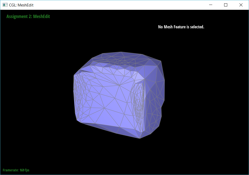
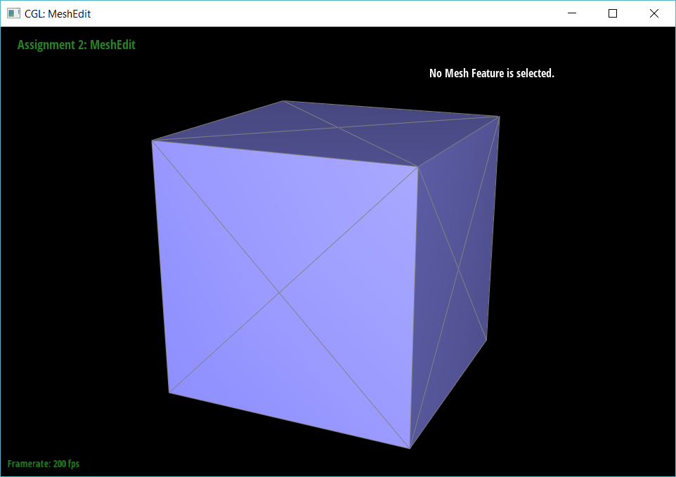
cube.dae becomes slightly asymmetric after repeated subdivision steps (as seen in the images of meshes after Loop subdivision). This is because the original mesh was asymmetric, so vertices did not necessarily have the same degree (number of neighbors). Differering degrees means means the delta (change in position) varies among vertices. If we pre-process the cube with flip and split to make the starting mesh more symmetrical, we can have it subdivide symmetrically. Specifically, we could split the diagonal edge on each face to ensure that all corner vertices have the same degree and all center vertices (center of the face) have the same degree. This ensures the deltas (change in positions) among the corner vertices/center vertices are the same, allowing us to subdivide symmetrically. See below for examples:

Section III: Mesh Competition

Part 7: Design your own mesh!

I haven't made the mesh yet but I'm gonna do it before the art competition submission deadline.