In this project I generated rays, tested for ray intersections with primitives (triangles and spheres), constructed bounding volume hierarchies to speed up the intersection tests, and implemented some cool illumination techniques. Specifically, I implemented direct and indirect illumination, and at the end of the project, I also implemented adaptive sampling to eliminate noise in the rendered images. Combined, these parts form the core components of a physically-based renderer using a pathtracing algorithm.
Part 1: Ray Generation and Intersection
To generate rays, I implemented the function generate_ray(x,y), which generates Ray objects with origin at the camera’s position. The direction of the ray is specified by the parameters x and y. Since the parameters x and y are within the range [0,1], I used two field of view angles to help me define my ray’s direction in camera space. Specifically, I defined a sensor plane one unit along the view direction where Vector3D(-tan(radians(hFov)*.5), -tan(radians(vFov)*.5),-1) was the bottom left and Vector3D( tan(radians(hFov)*.5), tan(radians(vFov)*.5),-1) was the top right of the sensor plane. Then, I mapped the input point’s x and y such that input point (0,0) maps to the bottom left and input point (1,1) maps to the top right. I accomplished this mapping by using a simple interpolation equation: Vector3D(topright.x - botleft.x) * x + botleft.x, (topright.y - botleft.y) * y + botleft.y, -1.0). Finally, by applying the transform c2w (camera to world), I was able to convert the direction vector to world space.
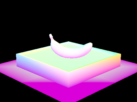
After creating generate_ray(x,y), I was able to cast rays starting at the origin. In raytrace_pixel(x,y), the paramaters x, y represent the coordinates of a pixel (specifically the “bottom left” of a pixel). Then, I sent ns_aa rays that pass through the pixel at random locations by using a small offset value. However, simply creating rays is not enough to render the scene. Thus, in the next part of the project, I implemented the primitive intersection parts of the rendering pipeline.
In this project, I implemented triangle and sphere intersection. These methods allow us to detect if the ray intersects objects. For triangle intersection, I used the Moller Trumbore algorithm. Essentially, by substituting the ray’s intersection point (P in the equation P = o +tD) with its barycentric form (alpha*P1 + beta*P2 + (1-alpha-beta)*P3), we can simplify the equation in such a way to obtain the barycentric coordinates and t intersection value. Specifically, if we change the equation to matrix form such that t, alpha, beta are the solutions, we can then use Cramer’s rule (which involves various dot products) to get the solution values t, alpha, beta.
Finally, to test if the solutions indicate an intersection, I check the following conditions: if alpha, beta, or gamma is less than 0, there is no intersection. If t is greater than r.max_t or less than r.min_t, there is no intersection. If the solutions don't fall under those categories, there is an intersection and I would update r.max_t to t. Then, I either return true or update the intersection (if an intersection struct was passed in to the function). I update the intersection to include the t value of the intersection, the normal, the intersected primitive, and the BSDF.
I also implemented sphere intersection. Here, I used the quadratic formula to get the t value, where "a" equals the direction vector * direction vector, "b" equals 2*(ray origin - center of sphere)*direction, and "c" equals (ray origin - center of sphere) * (ray origin - center of sphere) - (radius of sphere)^2. If the discriminant in the quadratic formula is less than 0, I return false. If the discriminant in the quadratic formula is greater than or equal to 0, I obtain t1 and t2 and check if t1 is less than min_t and t2 is greater than max_t. If so, return false. Else, return true as they are in the desired range.

|

|
|
Part 2: Bounding Volume Hierarchy
To construct the BVH, I first computed the bounding box containing the primitives and created a BVH node. If the number of primitives in vector
Now I will walk through my BVH intersection algorithm. If the ray misses the bounding box, return false. AS a side note, I was able to determine the intersection of the bounding box by using the simple ray and axis-aligned plane intersection equation described in lecture. Essentially, I recorded the min and max t values in each dimension (x, y, z), and found the min of the max t's and max of the min t's to determine the range. Moving on, if the ray hits the bounding box, we need to check if it hits any primitives. To do this, I first check if the current node is a leaf node. If not, I recursively call the right and left child of the node. Once we reach a leaf node, I iterate through all the primitives, checking if the ray intersects any of the primitives. If it intersects a primitive, return true.

|

|
|
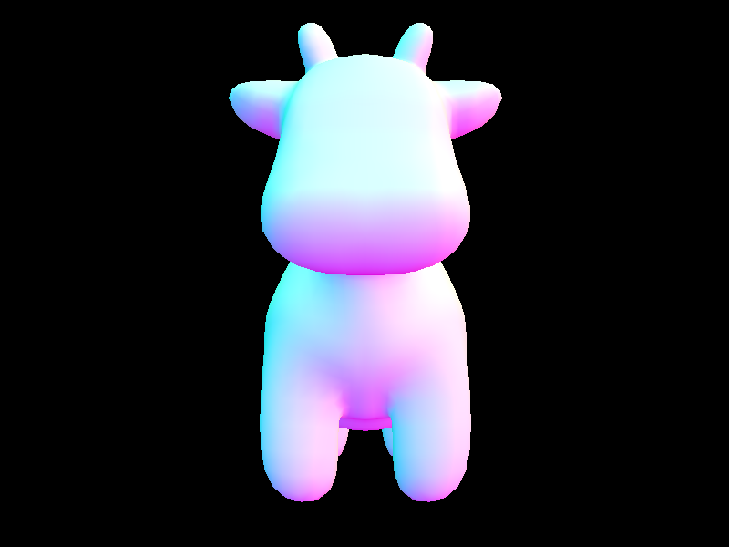
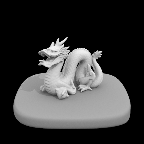
The cow above took 390 seconds to load before implementing BVH and had an average of around 3270 intersection tests per ray. After constructing the BVH algorithm, the cow only took 0.3554 seconds to load and had an average of 8 intersection tests per ray! The CBSpheres_lambertian (image shown in part 1) took .35 seconds before BVH, and .15 seconds after implementing BVH. Note this difference is smaller than in cow.dae since there are less primitives in CBSpheres_lambertian (only 14 primitives). BVH speeds up the pathtracer because we don’t need to check if a ray hits every primitive. Instead, we can narrow it down to a smaller bounding box, and see if it the ray hits only the primitives within that box. Thus, we test ray intersection on a smaller amount of primitives (compared to pre-BVH).
Part 3: Direct Illumination
In part 3, I implemented two different direct lighting estimations. My first method was to estimate the direct lighting of a point by sampling uniformly at random in a hemisphere. The second approach sampled from the lights directly.
To implement direct lighting sampling from the hemisphere, I iterated num_samples amount of times on the follow procedure: first, I sampled a random direction from the intersection point and converted it to world space. Then, I set this sampled direction as a new ray’s direction. I cast this new ray into the scene from the hit point (plus a tiny adjustment to make sure the ray avoids floating point imprecision) and check if this ray intersects with anything. If there is an intersection, I add the light output contribution from that intersected point (obtained by multiplying the emitted light by the bsdf and the wi.z to get the proportional contribution to the light output and take into account the direction from the normal). Finally, I divide this resulting value by the PDF (performing Monte Carlo integration) to carefully weight the results. After iterating this procedure num_sample times, I divide L_out by num_samples to get the average.
I also implemented importance sampling by sampling over the lights directly. This approach differs from uniform sampling in that it only samples directions that point towards a light source. Thus, I iterated through the lights and obtained directions pointing at those light areas (or one direction if the light is a single point). I then cast these shadow rays from the hit point and check to see if it hits any primitives. Critically, if it hits a primitive, I discard the sample! This is because if the ray hits a primitive before hitting the light, it is not reaching the light directly from the hit point. If it not does intersect with a primitive, I add the contributing irradiance from the light source (obtained by multiplying the incoming radiance by the bsdf and the wi.z to get the proportional contribution to the light output and take into account the direction from the normal). Finally, I divide this resulting value by the PDF (corresponding to this cast ray) and average the result by dividing by num_samples.
Below are some images rendered with both implementations of the direct lighting function.

|

|

|

|
|
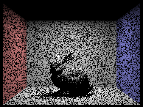
Below I focus on one particular scene (with at least one area light) and compare the noise levels in soft shadows when rendering with 1, 4, 16, and 64 light rays (the -l flag) and 1 sample per pixel (the -s flag) using light sampling, not uniform hemisphere sampling. As you can see below, increasing the number of light rays makes the image clearer and less noisy. This is because increasing the number of light rays ensures we have a "sufficient" number of shadow rays that are hitting the light source rather than intersecting an object before hitting the light source.
|
|

|

|
Now I will compare the results between using uniform hemisphere sampling and lighting sampling. Uniform hemisphere sampling creates more noise because its sampling technique is uniformly random, so the sampled rays don't always intersect with an object. Thus, although uniform hemisphere sampling will eventually converge to the correct image, it will be really slow. Furthermore, uniform hemisphere sampling can't render scenes with point light sources because it is extremely unlikely a sample will directly hit the point light source. Lighting sampling on the other hand samples directly from the light source. This ensures that we won't be shooting out unnecessary rays to random areas (although some of these shadow rays may be intersected by an object on its way to the light source), which means that this approach is more optimal. These differences can be seen in the images at the beginning of Part 4, where lighting sampling produces much clearer/less noisy images than uniform hemisphere sampling.
Part 4: Global Illumination
In part four, I implemented indirect lighting. Starting with the simplest function, I implemented zero_bounce_radiance, which returns the light emitted by the given point (zero for non-light sources). Next, I implemented one_bounce_radiance. This is equivalent to the direct illumination implementation from Part 3. Finally, I worked on at_least_one_bounce_radiance, which calls one_bounce_radiance and recursively calls itself to estimate more bounces. In each recursive call, there is a probability of 0.3 (I set the Russian Roulette probability to 0.7) the path may terminate. If it doesn’t terminate, I simply cast a sample ray from the current hit point and obtain the irradiance from an intersect point (using the same equation as in part 3 to calculate irradiance except additionally dividing by my Russian Roulette probability and performing the recursive call on the radiance). Also, if the number of recursive calls surpass max_ray_depth, I terminate the path tracing.
Below are some images rendered with global (direct and indirect) illumination. I used 1024 samples per pixel.

|
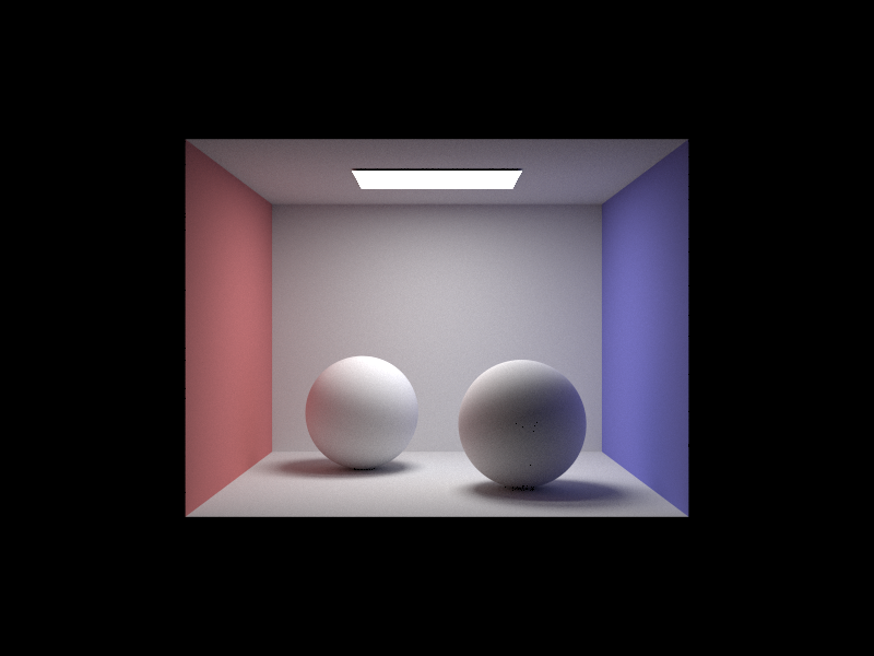
|
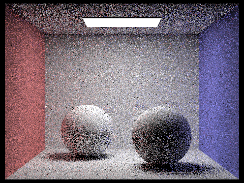
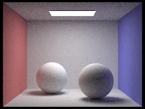
Below I pick one scene (spheres) and compare rendered views first with only direct illumination, then only indirect illumination. I used 1024 samples per pixel.
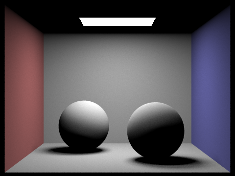
|
|
The direct only image was rendered using one_bounce_radiance (+ zero_bounce_radiance ) while indirect only calls at_least_one_bounce_radiance (+ zero_bounce_radiance) but skips the first call to one_bounce_radiance inside at_least_one_bounce_radiance.
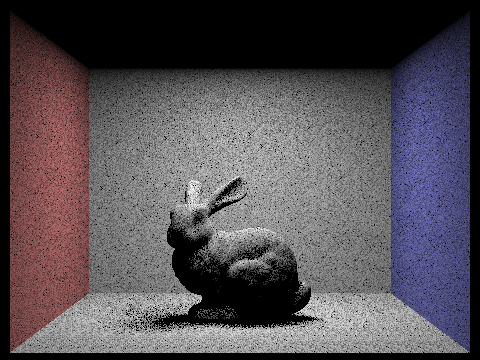
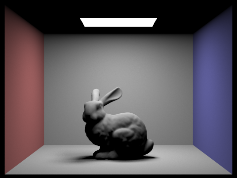
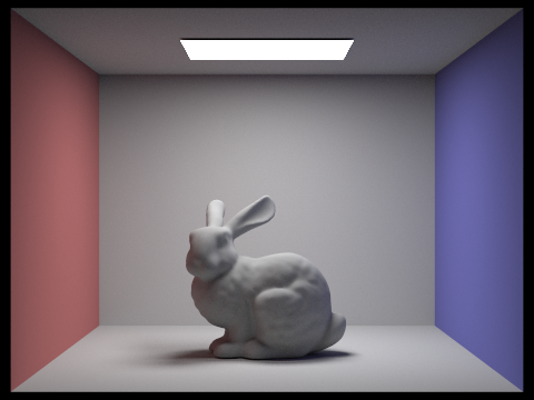
Below I compare rendered views of CBbunny.dae with max_ray_depth equal to 0, 1, 2, 3, and 100 (the -m flag). I used 1024 samples per pixel and 4 light rays.
|

|
|
|
|

|
As you can see above, the images become brighter/clearer as the depth increases. This is because as the depth increases, we can model more light bounces, which leads to more realistic lighting.
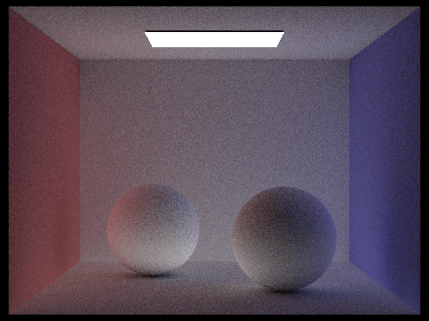
Below I pick the sphere scene and compared rendered views with various sample-per-pixel rates, including 1, 2, 4, 8, 16, 64, and 1024. I used 4 light rays.
|

|

|

|
|

|

|
As you can see above, the spheres become a lot less noisy with the samples increase. This is expected because increasing the sample rate helps us more accurately determine the light outputted at a specific point.
Part 5: Adaptive Sampling
In part 5, I implemented adaptive sampling to help eliminate noise in rendered images. This how it works: after samplesPerBatch of pixels, I obtain the mean and variance of the samples calculated so far. Then, I check if the following equation is true: 1.96*sqrt(sigmasquared / samplessofar) <= maxTolerance * mu. If its true, the pixel’s illuminance has converged and I stop looping. Otherwise, I continue tracing the ray and updating the s1 and s2 values (which are used in the mean and variance calculation) until I accumulate enough samples again such that samplessofar%samplesPerBatch == 0. Then I test convergence again by using the max tolerance equation listed above.
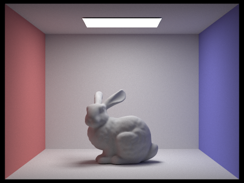
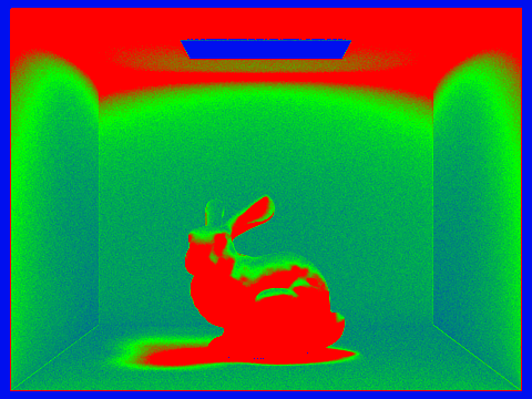
Below I pick one scene and render it with 2048 samples per pixel. I also show a sampling rate image with clearly visible differences in sampling rate over various regions and pixels. I used 1 sample per light and 5 for max ray depth.
|
|