Overview

In this assignment, I implemented a simple rasterizer, including features like supersampling, hierarchical transforms, and texture mapping with antialiasing. At the end, I have a functional vector graphics renderer that can take in modified SVG (Scalable Vector Graphics) files, which are widely used on the internet.

Section I: Rasterization

Part 1: Rasterizing single-color triangles

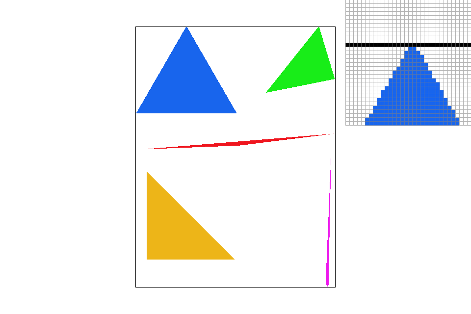
I rasterized the triangle by iterating through the (x,y) coordinates found within the bounding box of the triangle . To create this bounding box region, I obtained the minimum and maximum X and Y values from the given three triangle vertex coordinates. Then, I iterated through these points by using a nested for loop that goes from min X to max X and min Y to max Y. Thus, this algorithm is no worse than one that checks each sample within the bounding box of the triangle. For each sample point within this bounded region, I utilized the Three Line Test to determine if the sample point is within the triangle. Finally, if the point was inside, I filled it with a color. Below is a screenshot of the test4.svg file, with the pixel inspector centered on an interesting part of the scene.

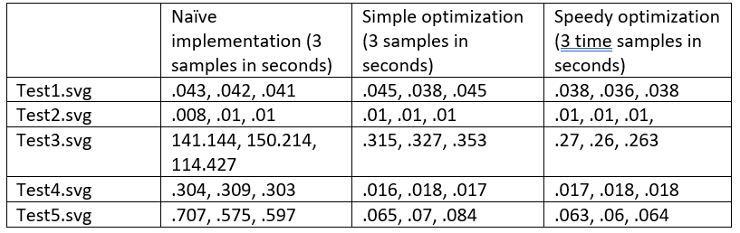
Extra Credit: Initially, I implemented my triangle rasterizer by scanning through every pixel in the sample buffer. This caused images to load very slowly, which was particularly noticeable in Test3.svg. My first step in optimizing the triangle rasterizer was to limit the size of the scanning region to the bounding box of the triangle and factor out redundant arithmetic operations used in the Three Line Test. The results of these optimization can be seen in the "Simple optimization" column in the time comparison table below. It should be noted I used clock() and CLOCK_PER_SEC in the redraw function to record loading time. As you can see, the various optimizations create an extremely noticeable difference in loading time for Test3.svg. To further optimize my rasterizer, I came up with an approach that allows the triangle rasterizer to skip certain pixels that do not need to be visited. Observe the following cases. In a single row, a sample point is either:

• left of the triangle
• inside the triangle
• right of the triangle

Thus, for each row, I tracked two specific boolean variables: whether any sample point in the row has been determined to be inside the triangle and whether a sample point is to the right of the triangle (the second boolean comes from the fact that I am scanning from left to right). The key idea is that if the rasterizer has found sample points within a triangle, then the next point (lets call it "point X") that is not within the triangle would indicate the scanning process has "exited" the triangle and is now to the right of the triangle. This means that any point to the right of "point X" is also to the right of triangle. Thus, by keeping track of these booleans, I was able to further optimize the triangle rasterizer and skip unnecessary sample points to the right of a triangle. The optimization times are shown in the last column of the table below.

Part 2: Antialiasing triangles

In Part 2 of the project, I used supersampling to antialias my triangles. Supersampling is very useful as it captures more high frequency information, providing smoother transitions between pixels and thus helps remove various aliasing artifacts, such as jagged edges. I modified my rasterization pipeline to account for the supersampling sample_rate; for each pixel in the region of interest, I divided them into a “sample_rate” amount of sub-pixels and then averaged the colors from the sub-pixels. It is important to note that the point-triangle tests was performed for each of the sub-pixels (using the center of the sub-pixels as the testing coordinate); this is important because whether or not a sub-pixel is in a triangle would affect the overall color of the entire pixel. By averaging these sub-pixel colors, I was able to produce a smoother image with less jagged edges.

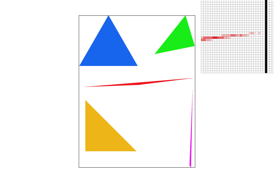
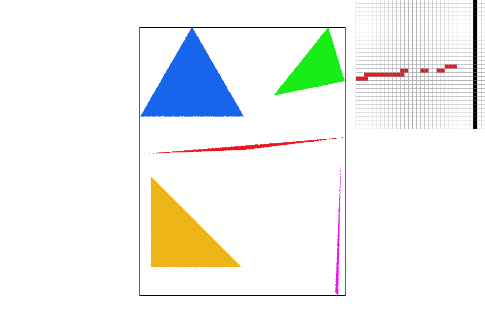
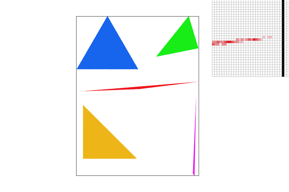
Below are screenshots of the test4.svg file with the sample rates set at 1, 4, 9, and 16. The pixel inspector is set to the corner of the thin red triangle to clearly show the visual affect of changing the sample rate. As you can see, as the sample rate increases, the thin corner of the triangle becomes more connected (there are less isolated points) and smoother overall. This is because by averaging the sub-pixel colors, we can get different shades of red (instead of distinctly one shade of red versus white in this particular triangle). The gradual change in colors/shading creates a smooth transition in pixel colors.

Extra Credit: For extra credit, I implemented jittered sampling. Jittered sampling is essentialy supersampling except when we perform the point-triangle tests, we perform it on a random point within the sub-pixel rather than the center of the sub-pixel. Jittered samples could improve the overall quality of the image when the jittered samples are well-distributed over the pixel. This is evident in the screenshots below, where the jittered sampling appears extremely jagged at low sampling rates, but becomes increasingly smooth at higher sampling rates. For example, the image at a jittered sampling rate of 4 has a connected edge (no island pixels), while the image depicted using a grid-based sampling rate of 4 has an isolated pixel at the very corner.

Part 3: Transforms

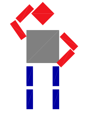
My robot image depicts a man scratching his head, deep in thought. I translated and rotated his left arm components so that he is scratching his head and thinking. I translated and rotated his right arm components so that his hand is on his waist to emphasize he is deep in thought. I also changed the color of his legs to blue so that it seems like he is wearing jeans, and changed his torso to grey so that he is wearing a shirt.

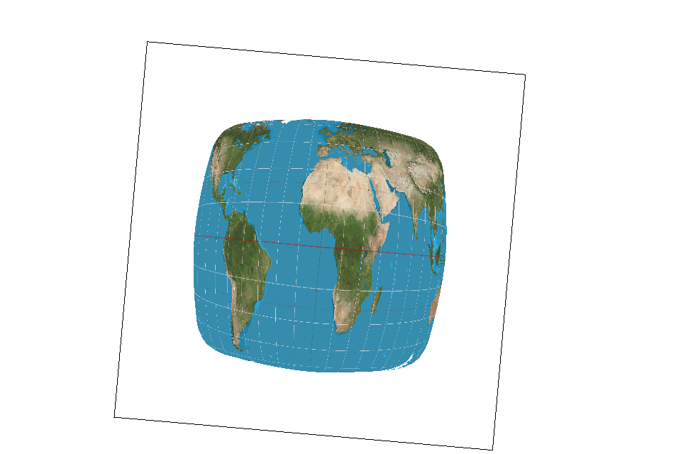
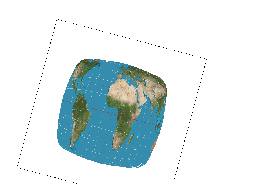
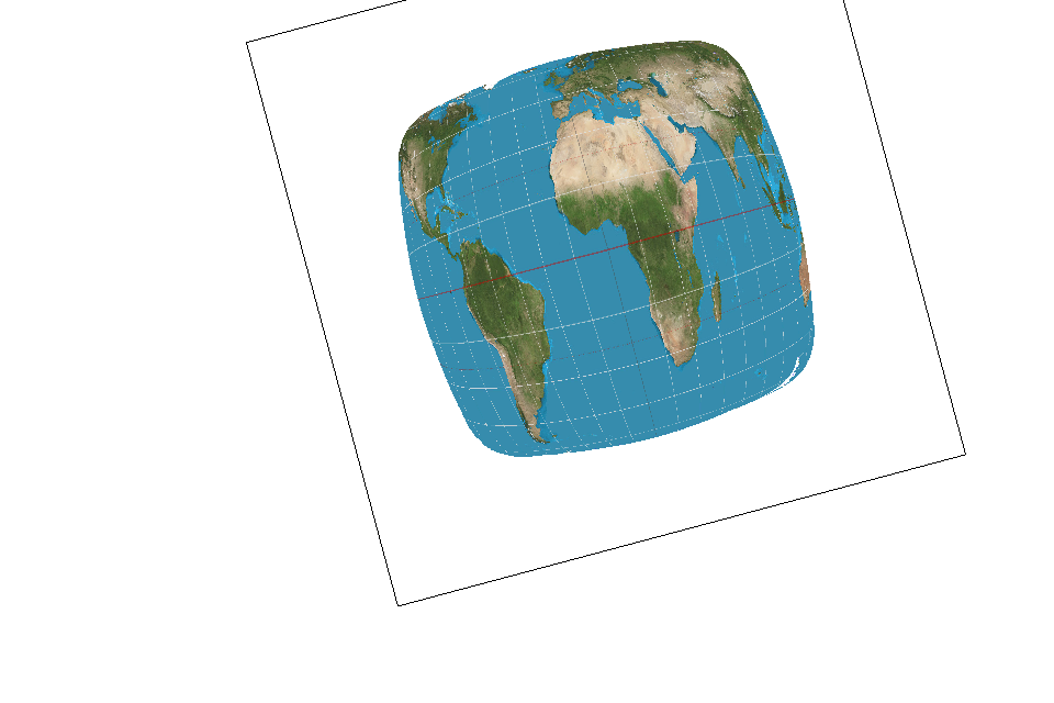
Extra credit: I rotated the viewport by multiplying the svg_to_ndc[current_svg] matrix with the rotation matrix. To prevent the viewport from resetting to its default matrix when pressing other keys, I added a rotation angle parameter to the set_view function and changed all calls to set_view to include a rotation angle argument. The rotation angle argument is set to be the "viewportradianangle" global variable, which has a default value of 0. The "[" and "]" keys increase/decrease this global variable by 5 degree.

Section II: Sampling

Part 4: Barycentric coordinates

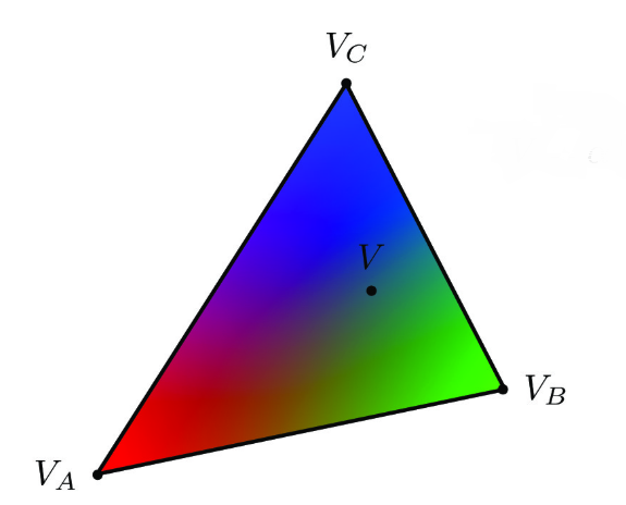
I used barycentric coordinates to linearly interpolate colors between vertices of a triangle. By getting the barycentric coordinates (alpha, beta, gamma weights) for a sample point, I was able to find and assign the weighted average of the vertex colors to each sample point location within a triangle. For example, in the smoothly blended triangle below (image is from CS 184 Lecture 5), each triangle vertex is initially assigned a color: A (V_a) is red, B (V_b) is green, and C (V_c) is blue. Given a sample point (x,y) within the triangle, the point’s color is equal to alpha*A + beta*B + gamma*C. Thus, my main task for this part of the project was to find the correct alpha, beta, gamma weights. I did this by utilizing the following equations: Alpha = Line equation for edge BC (x,y)/Line equation for edge BC (x_A,y_A). Beta = Line equation for edge CA(x, y)/ Line equation for edge CA (x_B,y_B). Gamma = 1 – Alpha – Beta. As you can see below, by interpolating across the triangle, I was able to specify weighted colors at each sample point and obtain a smooth transition of values across the surface.

Part 5: "Pixel sampling" for texture mapping

In part 5, pixel sampling is the process of evaluating a function at a sample point in order get its corresponding color from the texture space. To implement this, I used barycentric coordinates of the sample point and applied those weights (alpha, beta, gamma) to the per-vertex uv coordinates. This returned the appropriate uv coordinates of the sample point. Then, to determine the correct texture color for the uv coordinate, I implemented two different sampling algorithms: nearest sampling and bilinear sampling. Nearest sampling is very simple to implement because all it does is select the color value of the nearest texel (relative to the uv coordinate). However, nearest sampling is not very accurate because sometimes many texels contribute to the pixel footprint or many pixels cover a texel (this happens during minification and magnification), and the nearest sampling algorithm would still look at only one texel. The second algorithm, bilinear sampling, mitigates some of these issues by taking four neighboring sample locations and interpolating their colors to get the weighted average color . This resulted in a smoother image overall, removing some of the aliasing affects that result from magnification and minification.

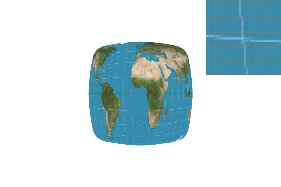
Below are examples of nearest and bilinear sampling. Lower sampling rates have more aliasing artifacts (e.g jaggies) than higher sampling rates. Bilinear sampling reduces the amount of aliasing artifacts by smoothing out the image. Shown below, the zoomed in areas of the bilinear images depict a solid line, while the nearest pixel sampling images depict a disconnected line with many components. This is because nearest sampling only looks at the nearest texel, so it may not receive the proper mapping value. On the other hand, bilinear sampling computes a weighted average of neighboring colors, which helps reduce the amount of frequency-related distortions. However, it should be noted that bilinear may make an image overly blurry if the image was extremely magnified.

As expected, the image below with the most aliasing artifacts is the nearest-pixel sampling with sumpersampling at 1, and the "smoothest" image is the bilinear sampling with supersampling at 16. Large differences between nearest-pixel and bilinear sampling occur when it's sampling pixels near thin lines. This difference is depicted in the zoomed in areas below. Nearest pixel sampling can assign the incorrect color to a pixel because the pixel is simply mapped to the nearest texel. It should be noted that bilinear sampling is a lot slower than nearest sampling because it requires more computation to determine the texture color for a pixel.

Part 6: "Level sampling" with mipmaps for texture mapping

Level sampling involves sampling from different mipmap levels. This allows for the use of different levels of detail according to the distance between object and viewpoint, which is useful in situations where a single pixel maps to multiple pixels in the texture map. For example, If the screen pixel is mapped to a texture coordinate that is far away, then switching to a higher MipMap level can help convey the perspective better. To calculate the appropriate MipMap level, I obtained the difference vectors by observing how far away the points (x, y+1) and (x+1, y) were in the texture plane. Specifically, I calculated the uv coordinates sp.p_dx_uv and sp.p_dy_uv by using the barycentric coordinates of (x, y+1) and (x+1,y). Then, I found the distance vectors (sp.p_dx_uv – sp.p_uv and sp.p_dy_uv – sp.p_uv). After scaling the distance vectors to the texture width/height, I used the following log equation: L = max(sqrt((du_dx * du_dx)+(dv_dx * dv_dx)),sqrt((du_dy * du_dy)+(dv_dy * dv_dy))) to determine the level. As discussed earlier, if the distance is large, get_level would output a relatively high mipmap level. If the distance is small, than it would use a smaller mipmap level. Since the output level is typically not an exact integer, we round to the nearest level or interpolate the color from the lower and upper level depending on our intended method (nearest level sampling vs bilinear level sampling).

Using level sampling, pixel sampling, and number of samples per pixel help smooth out the image and increase the overall antialiasing power of the program. However, these techniques often take some time to execute. This is because the program must compute arithmetic operations and loop through the pixels within the triangle. Bilinear takes longer to execute than nearest level/ nearest pixel sampling because it must compute the nearest neighbors' values and perform more rigorous calculations. Lastly, increasing the sample rate also takes up more memory because you have to loop through the pixels sample_rate more times (each pixel is divided into sample_rate subpixels). It should be noted the affects of these techniques can compound each other. For example, bilinear level sampling combined with bilinear sampling is the slowest and best at antialiasing in this project. In summary, the tradeoffs are as follows:

Techniques	Pros	Cons
Bilinear Level Sampling	Largest antialiasing power out of level sampling options in this project	Slowest because need to check neighboring values
Nearest Level	Less antialiasing artifacts than level 0 sampling	Slow, lower antialiasing power than bilinear because doesn't look at neighboring values
Level 0 Sampling	Decent speed	Least antialiasing power among level sampling techniques, uses a lot of memory because doesn't use mipmaps
Nearest-Pixel Sampling	Decent speed	Not always accurate because sometimes many texels contribute to the pixel footprint , least antialiasing power among pixel sampling techniques
Bilinear Sampling	Largest antialiasing power out of pixel sampling options in this project	Slowest

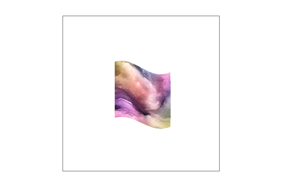
The above images of a galaxy depict the combination of the following techiniques: [level zero sampling, nearest level sampling] and [nearest pixel sampling, bilinear pixel interpolation sampling]. Although the affects of the techniques aren't too clear in this particular image, nearest level sampling combined with bilinear pixel interpolation sampling should have the smoothest overall look.

Section III: Art Competition

I haven't made the svg yet but I'm gonna do it before the art competition submission deadline.

Part 7: Draw something interesting!